Vanoxerine conc-QTc analysis

This case study demonstrates how to assess cardiac safety through conc–QTc modeling using Monolix. It shows step-by-step how to build a concentration–QTc model from a clinical study, based on a vanoxerine dataset, and evaluate proarrhythmic risk in line with ICH E14 guidelines. The first section shows the standard approach using the pre-specified linear model via the use of the conc-QTc R package. The second section shows the development of a PK/QTc model, which is necessary when a delay is detected.

Download the case study material

Introduction and case study outline

The assessment of cardiac safety is a key component in drug development, as drug-induced QT prolongation can increase the risk of ventricular arrhythmias such as torsade de pointes. The QT interval, measured on an electrocardiogram, represents the time between ventricular depolarization and repolarization. Prolongation of this interval may be linked to early after-depolarizations and life-threatening arrhythmias.

Traditionally, the thorough QT (TQT) study was the standard to evaluate this risk. However, the 2015 revision of the ICH E14 Q&A document (R3) allows for concentration–QTc (C–QTc) modeling as a primary approach, using high quality electrocardiogram (ECG) measurements from single-dose or multiple-dose escalation (SAD/MAD) studies during early-phase clinical development. In this modeling approach, the upper bound of the 90% confidence interval of the predicted QTc effect at the highest clinically relevant concentration is compared to the 10 milliseconds threshold (ICH E14 Q&A R3, 2015). This shift enables a model-informed evaluation of proarrhythmic potential, particularly when a TQT study is not feasible (Garnett et al., 2017; Darpo et al., 2022).

This case study illustrates such an approach using vanoxerine (GBR 12909), a dopamine reuptake inhibitor previously evaluated in a human pharmacology study involving cocaine-experienced volunteers. The study explored the safety, tolerability, and pharmacokinetics of escalating oral doses. Here, we first apply the standard linear model of the Garnett. et al white paper using the MonolixSuite-based conc-QTc R functions. However, the exploratory plots show that the assumptions required to apply the linear model are not fulfilled, due to a delay between the drug concentration and the effect on QTc. To capture this delay, we develop a population PK/PD model and use simulations to assess the QTc liability of vanoxerine, in line with regulatory recommendations.

Standard approach with linear C-QTc model

Study design

This C-QTc case study is based on a clinical trial data of a human laboratory study of Vanoxerine (GBR 12909) – a dopamine uptake inhibitor developed to treat cocaine dependence. Its human trials were blocked at Phase II because patients under treatment showed prolongation of the QT interval.

The clinical study was a double-blind, placebo-controlled, dose-escalating trial designed to assess the safety, tolerance, and pharmacokinetics of multiple escalating doses of Vanoxerine in cocaine-experienced volunteers.

The original study involved three escalating oral doses of Vanoxerine, administered daily for 10 days. Participants were divided into treatment and placebo groups, with two individuals receiving placebo. Drug concentration (mg/L) was measured starting after the third dose. and QT interval measurements were collected for all participants.

Data collection from case report forms

The data was obtained from the National Institute on Drug Abuse (NIDA) database at NIDA-CPU-0002 study. The plasma GBR12909 concentration is obtained from the EXTLABS.csv file, the ECG data from the ECGPRFL1.csv file and the treatment groups from the RDMCODE.csv file. The following R code is used to read and merged this information into a single file.

library(dplyr)

# read placebo and treatment groups (50 or 75 mg)
# remove placebo individuals and individuals that did not meet inclusion criteria
TRT <- read.csv("../ascii-crf-files_nida-cpu-0002/RDMCODE.csv") %>%
  filter(XTRTMT!="" & XTRTMT!="Placebo") %>%
  select(c(SUBJID,XTRTMT))

# read ECG data
ECG <- read.csv("../ascii-crf-files_nida-cpu-0002/ECGPRFL1.csv") %>% 
  select(c(STUDYID, SUBJID, VISID, ECGHOUR, ECG12TM, ECGPR, ECGQT, ECGQRS, ECGRR)) %>%
  group_by(SUBJID, VISID) %>%
  mutate(TIME=c(0, 0.5, 1, 2, 3, 4, 6, 8, 12)) %>%                 # add time column (nominal times based on protocol)
  mutate(BASELINE=if_else(TIME==0,"Y","N")) %>%                    # add baseline column (Y or N)
  mutate(TRT=if_else(VISID=="DAY0","Placebo","Vanoxerine")) %>%    # add treatment column with "placebo" or "vanoxerine"
  ungroup() %>%
  right_join(TRT, by="SUBJID")                                     # keep only non-placebo individuals using right_join

# read concentration data
CONC_ngmL <- read.csv("../ascii-crf-files_nida-cpu-0002/EXTLABS.csv") %>% 
  filter(TESTNAME=="Plasma GBR Concentration") %>%    # keep only PK measurements
  filter(COLLDATE==11) %>%                            # keep only day 11 (only troughs on the other days)
  right_join(TRT, by="SUBJID") %>%                    # keep only non-placebo individuals using right_join
  filter(!(SUBJID=="284255" & TIMETEXT==758)) %>%     # remove one duplicate conc for this id
  group_by(SUBJID) %>%
  mutate(TIME=c(0, 0.5, 1, 1.5, 2, 2.5, 3, 4, 6, 8, 12)) %>% # nominal times based on protocol (more points for CONC compared to QTc)
  mutate(VISID="DAY11") %>%
  select(c(SUBJID,VISID,TIME,RESULT)) %>%
  rename(CONC = RESULT) %>%
  ungroup()
  
# merge ECG and conc data
ECG_CONC <- ECG %>% 
  left_join(CONC_ngmL, by=c("SUBJID","VISID","TIME")) %>%  # merge conc data
  mutate(CONC=if_else(VISID=="DAY0","0",CONC)) %>%         # put conc = 0 for day 0 (placebo)
  mutate(TRT = if_else(TRT=="Placebo","Placebo",if_else(XTRTMT=="GBR12909 50 mg", "Vanoxerine 50 mg", "Vanorexine 75 mg"))) %>%
  rename(VISIT=VISID, DOSEGROUP=XTRTMT)%>%
  select(c(STUDYID, SUBJID, VISIT,TRT, TIME, CONC, BASELINE, ECGPR, ECGQT, ECGQRS, ECGRR))

write.csv(ECG_CONC, file="Vanoxerine_data.csv", quote=F, row.names = F)

We obtain the following dataset structure:

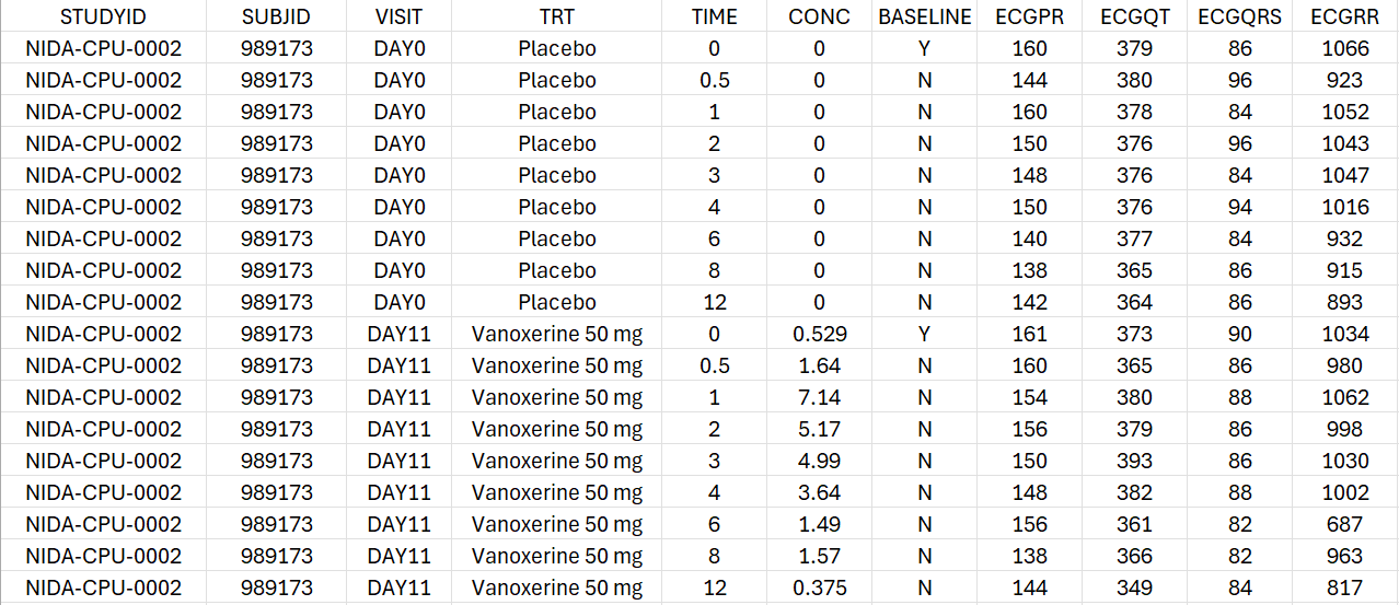
For each individual, the concentration and the PR, QT, QRS and RR intervals are measured on Day 0 under placebo treatment and on Day 11 under active treatment with either 50 mg or 75 mg of vanoxerine. For each period, the observations are recorded at time 0, 0.5, 1, 2, 3, 4, 6, 8 and 12 hours post-dose.

Data preparation for C-QTc analysis

In order to perform a concentration-QTc analysis and generate exploratory data analysis plots, it is necessary to apply the following processing steps:

• calculate heart-rate correction for QT to generate QTc, for instance using Fridericia’s formula

• calculate the baseline-corrected QTc, i.e ΔQTc. In our case, the baseline is simply the pre-dose measurement at time 0 hr. It is indicated in the dataset with BASELINE=Y

• given that both placebo and vanoxerine periods are available for each individual, it is also possible to calculate directly the baseline-corrected and placebo-corrected QTc, i.e ΔΔQTc

• for exploratory data visualization purpose, the ΔHR and ΔΔHR can also be computed

Covariates and regressor variables which will appear in the conc-QTc model must also be added as additional columns:

• BLQTc_cent: the centered QTc baseline

• BLQTc_centAdjPl: the placebo-adjusted centered baseline in case of ΔΔQTc

• TIME_cat: time as categorical factor

• Cc_reg: drug concentration

• RR_reg: RR interval duration (for plotting purpose)

These steps can be performed using the function process_QTcData() from the conc-QTc R functions.

First, the R script mlxQTcTools.R , which contains the conc-QTc related functions, must be sourced. In addition, to use these R functions, a MonolixSuite installation must be available and the lixoftConnectors R package installed. In order to indicate the location of the MonolixSuite installation, the functioninitQTc(path=...) is used.

source('../_mlxQTcTools/mlxQTcTools.R')
initQTc(path="C:/Program Files/Lixoft/MonolixSuite2024R1")

The process_QTcData() is called in the following way:

process_QTcData(data="Vanoxerine_data.csv", 
                QTname = "ECGQT", RRname = "ECGRR", CONCname = "CONC", 
                TRTname = "TRT", IDname = "SUBJID", TIMEname = "TIME", 
                placeboName="Placebo",
                bComputeBaseline = TRUE, BLFLAGname = "BASELINE",
                bComputeQTc = TRUE, correctionMethod = "Fridericia", 
                outName= "Vanoxerine_formatted.csv", silent= FALSE)

The column containing the QT, RR, drug concentration, treatment (placebo or drug), subject id and time are indicated using the arguments QTname, RRname, CONCname, TRTname, IDname, TIMEname. Note that the values present in the TRTname column will be used as plot labels for the report generation. If several dose levels are used, the TRTname column should contain different values for the different dose levels, for instance “Placebo”, “Vanoxerine 50 mg” and “Vanoxerine 75 mg”.

Given that the QTc column (heart rate-corrected QT) is not present in the dataset, it is computed using bComputeQTc = TRUE. Several correction methods are available and can be chosen. To use the most common Fridericia formula, we set correctionMethod = "Fridericia".

The QTc baseline column is not present yet in the dataset, so it is computed by setting bComputeBaseline = TRUE and indicating the baseline flag column in BLFLAGname. The baseline flag column should contain “0”/”1” values or “N”/”Y” values with “Y” and “1” indicating the baseline records.

The name of the output file is given via the outName argument.

Running the function generates the following console output, which details the applied formatting steps. This output can be supressed by choosing silent=T.

Info: The following treatment groups have been found: Placebo, Vanoxerine 50 mg, Vanorexine 75 mg
Info: The HR column has not been provided and has been calculated based on the 'ECGRR' column.
Info: The QTc column has been calculated based on the 'ECGQT' and 'ECGRR' columns, using Fridericia's formula: QTc=QT/(RR/1000)^(1/3)
Info: The BLQTc and BLHR columns have been calculated using the lines flagged as BASELINE=Y or 1.
Info: The dQTc and dHR columns have been calculated as dQTc=QTc-BLQTc and dHR=HR-BLHR.
Info: The BLQTc_cent column has been calculated as BLQTc_cent=BLQTc-mean(BLQTc).
Info: The ddQTc, ddRR and BLQTc_centAdjPl columns have be computed by subtracting the placebo data. 
Info: The Cc_reg (concentration as regressor), RR_reg (RR as regressor) and TIME_cat (TIME as categorical covariate) columns have been added.
 ==> Created new dataset Vanoxerine_formatted.csv. 

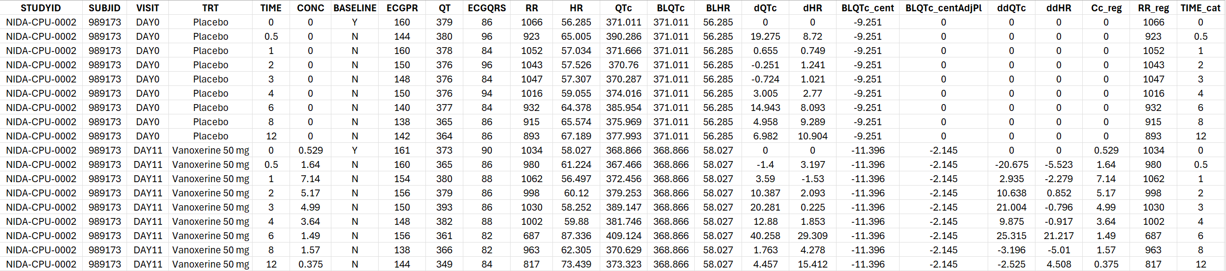
The generated formatted dataset has the following structure:

Standard C-QTc analysis

The standard C-QTc analysis proposed in the Garnett et al. White Paper uses a linear model for ΔQTc with concentration effect, treatment effect, time effect and centered baseline effect:

with i the individual, j the treatment and k the time. The parameters represent fixed effects and the terms indicate random effects.

If placebo data is available for each individual and ΔΔQTc can be calculated, as it is the case for Vanoxerine, ΔΔQTc can be modeled directly using a simpler model where the intercept and time points terms have cancelled out:

To run a C-QTc analysis for ΔΔQTc with this standard model, the function generateQTcProject() can be used:

generateQTcProject(dataSet="Vanoxerine_formatted.csv", 
                   IDname="SUBJID", TIMEname="TIME", TRTname="TRT", CONCname="CONC", 
                   placeboName = "Placebo", 
                   modelFile = "../_mlxQTcTools/models/ddQTcModels/model_ddQTc_Linear.txt", 
                   projectName = "./mlx_runs_linearOnly/ddQTc_Linear.mlxtran", 
                   isddQTC = TRUE, 
                   bRun = TRUE)

The user should provide the formatted dataset in the argument dataSet, as well as the name of the columns containing the subject id in IDname, time in TIMEname, treatment groups in TRTname, concentration in CONCname. The other columns (e.g QT, QTc, HR, etc) must have predefined headers and do not need to be specified. The category of the treatment group column representing placebo can be indicated using placeboName = "Placebo".

To select the standard linear model for ΔΔQTc, the file model_ddQTc_Linear.txt from the model library provided with the R functions can be used. The Monolix project will be saved as projectName = "./mlx_runs_linearOnly/Vano_standard_model.mlxtran".

Whether ΔΔQTc or ΔQTc is used must be indicated with isddQTC = T or F. To run the projects, use bRun = T. Given that each individual has a placebo period and ΔΔQTc could be computed, we model directly ΔΔQTc, which allows for faster runs.

Assessment of model assumptions

The following assumptions should be assessed to decipher the applicability of the standard linear model:

• Assumption 1: No drug effect on HR

• Assumption 2: QTc interval is independent of HR

• Assumption 3: No time delay between drug concentrations and ΔQTc or ΔΔQTc

• Assumption 4: Linear C-QTc relationship

Exploratory data analysis plots can be generated to assess these assumptions. This can be done via the generation of a report in Word format, based on a Quarto template. A Quarto template is provided as part of the R functions and can be used in the following way:

quarto_render(input = "../_mlxQTcTools/QTc_quarto_allModels.qmd", 
              output_file = "Vanoxerine_ddQTc_report_linear.docx",
              execute_params = list(folderName = "../Example_Vanoxerine/mlx_runs_linearOnly", 
                                    compoundName = "Vanoxerine",
                                    CONCname = "CONC", 
                                    placeboName = "Placebo", 
                                    studyType = "ddQTc",
                                    concentrationUnit = "ng/mL",
                                    nBins = 10))

The input argument give the path to the Quarto template, while the output_file is the generated Word report. The folderName gives the relative path from quarto template (.qmd) to folder containing the Monolix runs. Note that it is not the relative path from the current working directory but from the Quarto template. The compoundName and concentrationUnit will be used in the text and plot labels of the report, while placeboName should be the category of the treatment column representing the placebo individuals. The studyType can be dQTc (for ΔQTc) or ddQTC (for ΔΔQTc). The number of bins nBins will be applied in plots when binning of the concentration values is necessary.

The key diagnostic plots contained in the report are presented below. The entire report can be downloaded here.

Assumption 1: No drug effect on HR

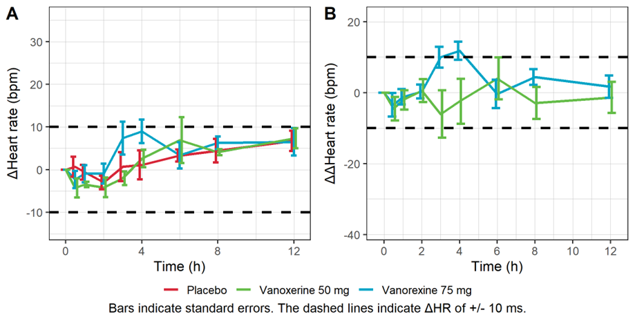
The figure below shows the time course of the mean heart rate stratified by treatment to assess a potential drug effect on heart rate. Although there is no consensus on the specific threshold effect on HR that could influence QT/ QTc assessment, mean changes of 10 bpm or more are considered problematic. The figure shows no significant effect of the drug concentration on ΔHR or ΔΔHR.

Mean baseline corrected (A) and baseline- and placebo-corrected (B) heart rate vs time.

Assumption 2: QTc interval is independent of HR

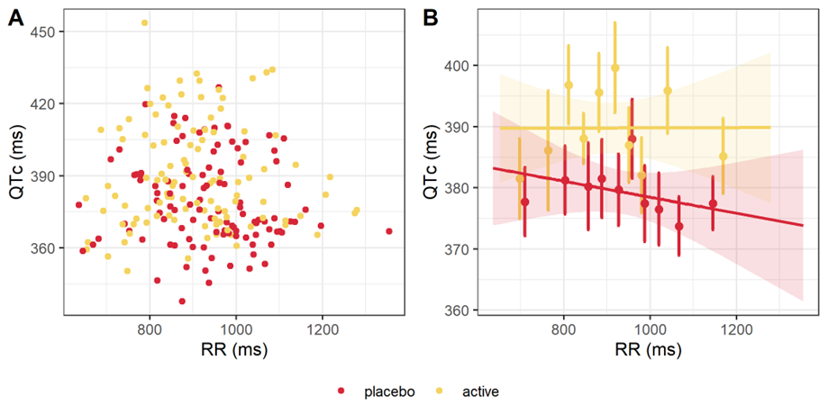
After heart-rate corrected, QTc is expected to be independent from the heart rate (HR) and from its inverse, the RR interval. A scatter plot of QTc interval duration vs RR interval duration, stratified by treatment, is provided below. The linear regression for the active and placebo groups are shown in panel B. The slopes are not significantly different from 0, with p-values being respectively 0.988 and 0.368. Thus, the QTc interval is independent from RR and from HR.

QTc interval duration vs RR, overall (A) and by treatment (B).

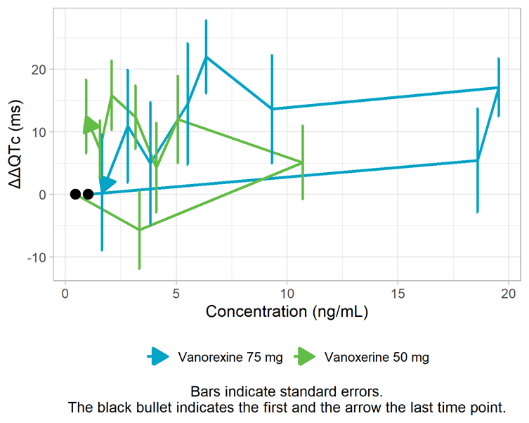
Assumption 3: No time delay between drug concentrations and ΔQTc

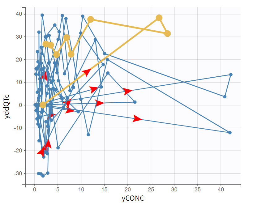
The assumption of a direct effect, i.e. an immediate change in ΔΔQTc following a change in concentration, is assessed visually below. With a direct effect, the effect increases and decreases with concentration on the same path. In the figure below, we observe a counterclockwise pattern which suggests the presence of hysteresis, i.e. a delayed effect. To investigate this assumption further, models with a delay will be explored in the next section “Alternative models”.

Mean ΔΔQTc per time point vs concentration

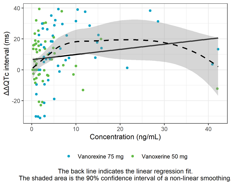
Assumption 4: Linear C-QTc relationship

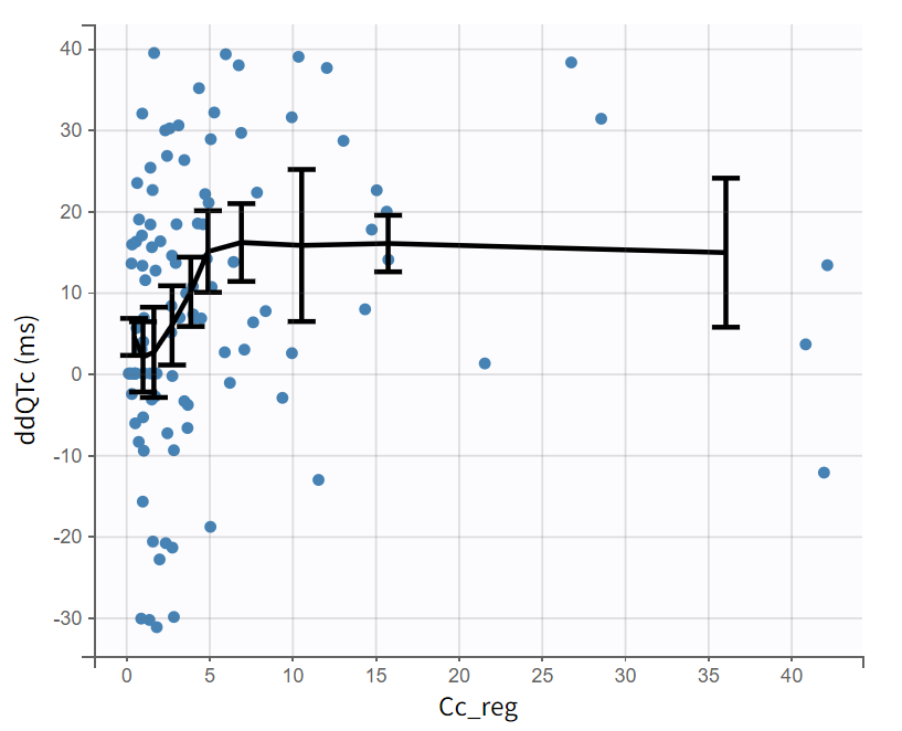
The linearity assumption between exposure and ΔΔQTc is assessed by a concentration-ΔΔQTc plot with linear regression and LOESS smoother. The shape of the LOESS smoother suggests that the relationship is not linear at high doses and that an Emax model might describe the data better. This will also be investigated further in the next section.

ΔΔQTc vs concentration

Alternative models

In the previous section, we have seen that the assumptions of no delay and linear relationship might not hold for the vanoxerine dataset. To explore this further, alternatives to the direct-effect linear model can be used.

It is possible to investigate other relationship shapes between drug concentration and ΔΔQTc (or ΔQTc) such as Emax, Emax with Hill coefficient, or log-linear. These models can be compared based on goodness of fit metrics such as the BICc. Furthermore, it is possible to assess if the introduction of a delay between the drug concentration and its effect on ΔΔQTc (or ΔQTc), via an effect compartment, improves the BICc. These alternative models are available in the library of models provided with the R functions.

To run all models present in the library, the function generateAllQTcProjects() can be used:

generateAllQTcProjects(dataSet="Vanoxerine_formatted.csv", 
                       IDname="SUBJID", TIMEname="TIME", TRTname="TRT", CONCname="CONC", 
                       placeboName = "Placebo", 
                       modelFolder="../_mlxQTcTools/models/ddQTcModels", 
                       projectFolder="./mlx_runs", 
                       isddQTC = TRUE, 
                       bRun = TRUE)

The arguments are similar to those of the generateQTcProject() function except that a modelFolder (containing the library models) and a projectFolder (containing the generated Monolix runs) argument are given.

The following output is generated in the console to follow the run progression and models tested:

Created project ./mlx_runs/ddQTc_Emax.mlxtran. Running project... Done.
Created project ./mlx_runs/ddQTc_Emax_effectComp.mlxtran. Running project... Done.
Created project ./mlx_runs/ddQTc_EmaxSigma.mlxtran. Running project... Done.
Created project ./mlx_runs/ddQTc_EmaxSigma_effectComp.mlxtran. Running project... Done.
Created project ./mlx_runs/ddQTc_Linear.mlxtran. Running project... Done.
Created project ./mlx_runs/ddQTc_Linear_effectComp.mlxtran. Running project... Done.
Created project ./mlx_runs/ddQTc_LogLinear.mlxtran. Running project... Done.
Created project ./mlx_runs/ddQTc_LogLinear_effectComp.mlxtran. Running project... Done.

To compare the results of the different models, a new report can be generated, which will provide comparison tables. The report is generated similarly to the first time. The only new argument is thresBICc to choose the threshold BICc value which will serve for the run comparison.

quarto_render(input = "../_mlxQTcTools/QTc_quarto_allModels.qmd", 
              output_file = "Vanoxerine_ddQTc_report_allModels.docx",
              execute_params = list(folderName = "../Example_Vanoxerine/mlx_runs",   # give relative path from quarto template (.qmd) to folder containing runs
                                    compoundName = "Vanoxerine",
                                    CONCname = "CONC", 
                                    placeboName = "Placebo", 
                                    studyType = "ddQTc",
                                    concentrationUnit = "ng/mL",
                                    nBins = 10,
                                    orderTRT = NULL,
                                    thresBICc = 0))

In the generated report, the presence of a delay is assessed by comparing the goodness of fit (via the BICc) of the standard linear model and a linear model with an effect compartment to introduce a delay. The table below shows that the model with effect compartment is 17 points better with a delay estimated to be 2.3 hours.

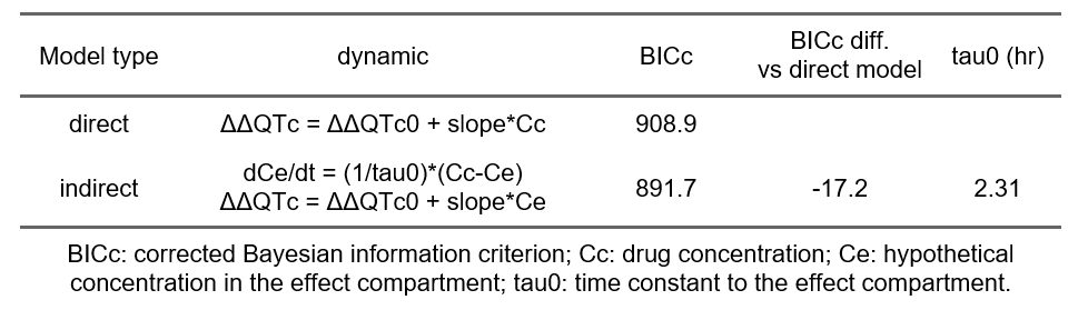
Thus, there is evidence of a delay between the drug concentration and its effect on ΔΔQTc. A delay might be caused by an active metabolite that exerts an effect on QTc such that the time delay between parent concentration and effect change actually describes the metabolism from parent drug to metabolite with the effect originating from the metabolite. In absence of knowledge or data on a possible metabolite, the delay can be described by an effect-compartment model (also called indirect model) for the observed drug concentration, as shown above.

In case of a delay, the time of maximum concentration may be substantially different from the time of maximum effect. The ΔΔQTc confidence interval cannot be derived using the usual formula anymore, where a range of Cc value is used to obtain the corresponding ΔΔQTc values. Indeed, the effect will not solely depend on the current concentration anymore but on the entire past profile of the drug concentration, as shown by the use of the time-derivative in the model. In order to obtain a ΔΔQTc confidence interval in case of a delay, it is necessary to develop a population PK/QTc model, that models not only the effect of concentration on QTc, but also the shape of the concentration over time. This is shown in the next section.

Even though a population PK/QTc model will be needed, we can nevertheless check the results of the alteratives models with different C-QTc relationship shapes:

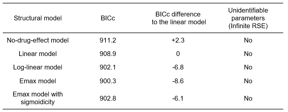
The comparison of the BICc goodness of fit metric indicates that an Emax model captures the data better (improvement of 8.6 points of BICc compared to the linear model). This is consistent with our observations based on the exploratory data analysis, and will guide the development of the population PK/QTc model.

Population PK-QTc model approach

Given that the immediate effect assumption required to apply the standard linear model is not fulfilled, it is necessary to develop a joined model capturing the PK concentration and its effect on the ΔΔQTc. In contrast with the standard approach where the observed drug concentration is used directly as model input (via a “regressor” in Monolix), in the PK/PD approach, the drug concentration is modeled and it is the model-predicted drug concentration which influences the QTc.

The previous section has shown that in addition to a delay, it is worth exploring different C-QTc relationship shapes, in particular an Emax model.

The development of the joint PK/ΔΔQTc model will be done in Monolix. In order to derived the ΔΔQTc confidence interval, Simulx will be used.

Data formatting

After having applied the process_QTcData() function, the dataset has the following structure:

• STUDYID: study id number

• SUBJD: patient id number

• VISIT: indicates the study day corresponding to each measurement (Day 0 or Day 11)

• TRT: categorical covariate to distinguish patients with “placebo”, “vanoxerine 50 mg” or “Vanoxerine 75 mg”

• TIME: measurement times (hours)

• CONC: measured Vanoxerine concentration (mg/L)

• BASELINE: flag indicating whether the time point corresponds to the baseline period (Y = baseline)

• ECGPR: measured PR segment (ms)

• QT: measured QT interval (ms).

• ECGQRS: measured QRS complex (ms)

• RR: measured RR interval (ms)

• HR: heart rate (beats per minute)

• QTc: QT interval corrected for heart rate (ms)

• BLQTc: corrected QT interval at baseline (ms)

• BLHR: heart rate at baseline (beats per minute)

• dQTc: change from baseline in QTc (QTc - BLQTc) (ms)

• dHR: change from baseline in HR (beats per minute)

• BLQTc_cent: baseline QTc interval, centered by subtracting the mean baseline QTc across all subjects (BLQTc_cent=BLQTc-mean(BLQTc)) (ms)

• BLQTc_centAdjPl: baseline QTc value, centered across subjects, and adjusted by subtracting the corresponding placebo value (BLQTc_centAdjPl = BLQTc_centTrtm- BLQTc_centPl)(ms)

• ddQTc: Baseline corrected and placebo adjusted QTc, defined as the difference between a subject’s dQTc on treatment and the corresponding dQTc on placebo (ddQTc = dQTc_Trtm - dQTc_Pl) (ms)

• ddHR: Baseline corrected and placebo adjusted heart rate (beats per minute)

• Cc_reg: measured Vanoxerine concentration (mg/L) to be used as a regressor

• RR_reg: measured RR interval (ms) to be used as a regressor

Given that we will work with ΔΔQTc which is placebo-corrected, we don’t need the rows corresponding to VISIT = DAY 0. Filtering out this part of the dataset in Monolix is possible but inconvenient (due to the occasion column which will remain after filtering, even if it is not needed). Instead we filter the dataset outside of Monolix and keep only the rows corresponding to VISIT=DAY 11.

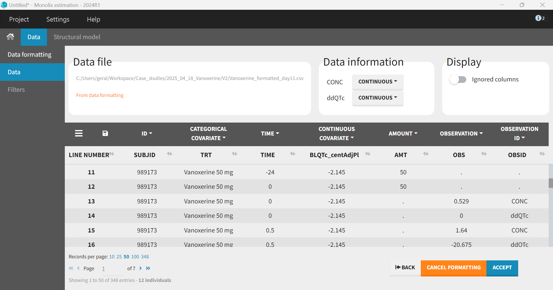
In order to use this dataset to develop a joined PK/PD model, the following modifications must be applied, via the data formatting module in Monolix.

• Merging the two observations of interest—Vanoxerine concentration (CONC) and baseline-corrected, placebo-adjusted QTc (ddQTc)—into a single observation column, and adding observation ID column to distinguish between them;

• Adding information on dose administration.

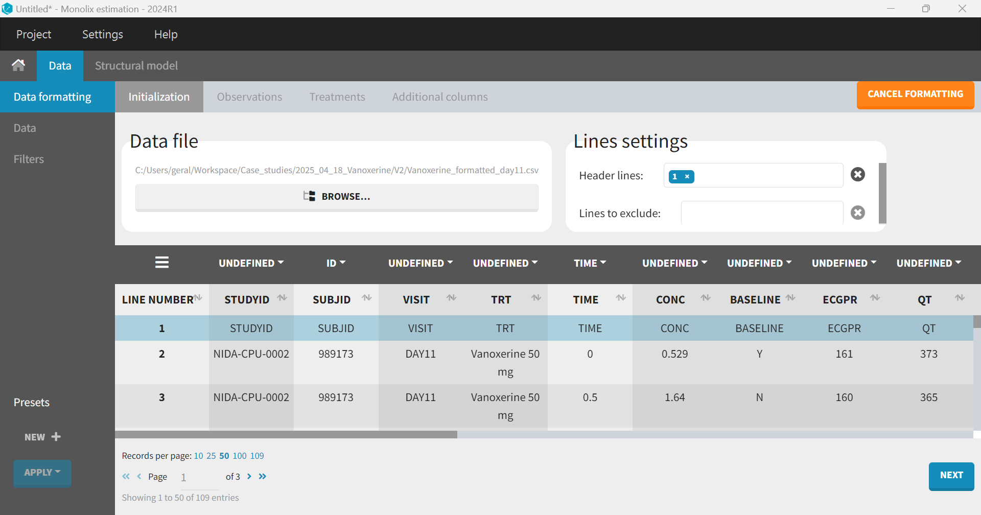
After having opened Monolix, the dataset is loaded directly through the data formatting module. The first step is the “Initialization” to specify columns that will define unique observations. In this case, the column SUBJID is tagged as “ID”, and TIME as “TIME”.

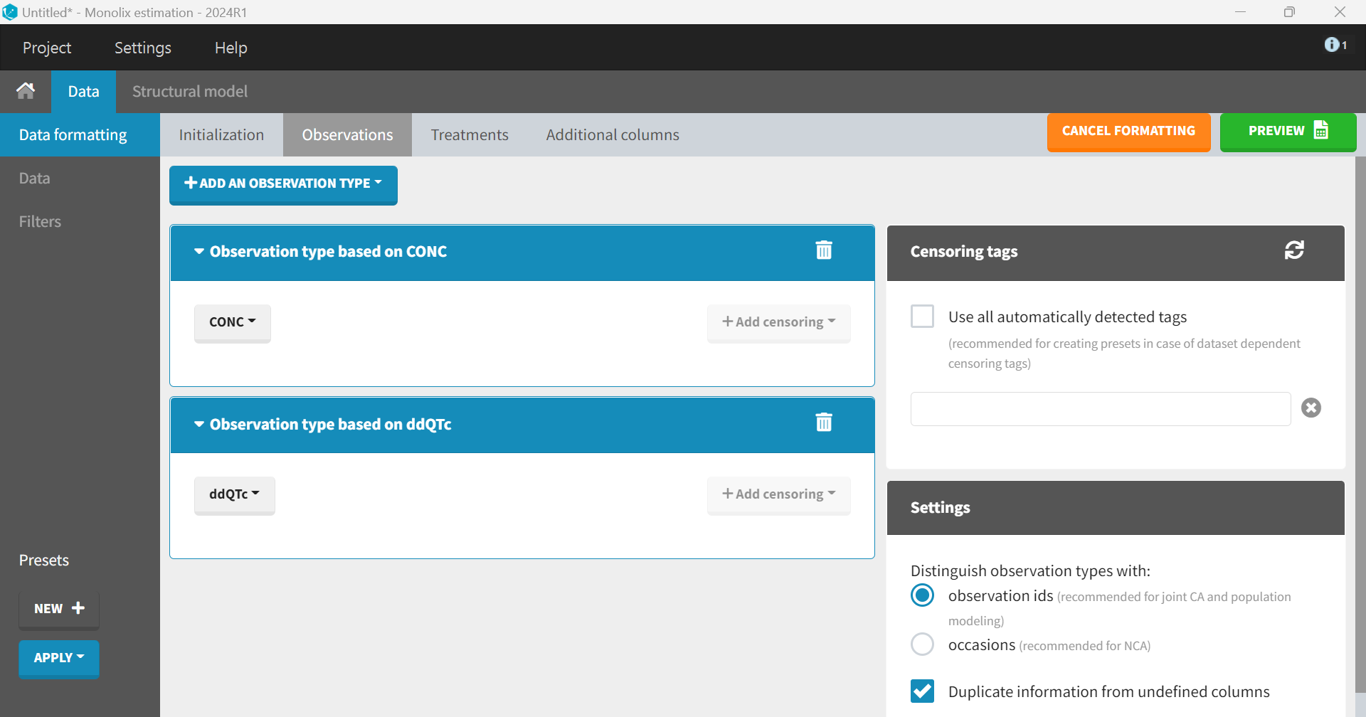
Clicking “Next” leads to the “Observations” tab. The dataset contains two separate columns with different types of observations, CONC and ddQTc, which should be combined into a single column. To do this, “+ Add an observation type” is selected, and CONC is chosen from the dropdown menu. The same step is repeated for ddQTc. The setting box, which appears on the right, allows to distinguish between the two observation types—either via an observation ID or via occasions. The default option “observation ID” should be selected in the case of joint PK/PD modeling.

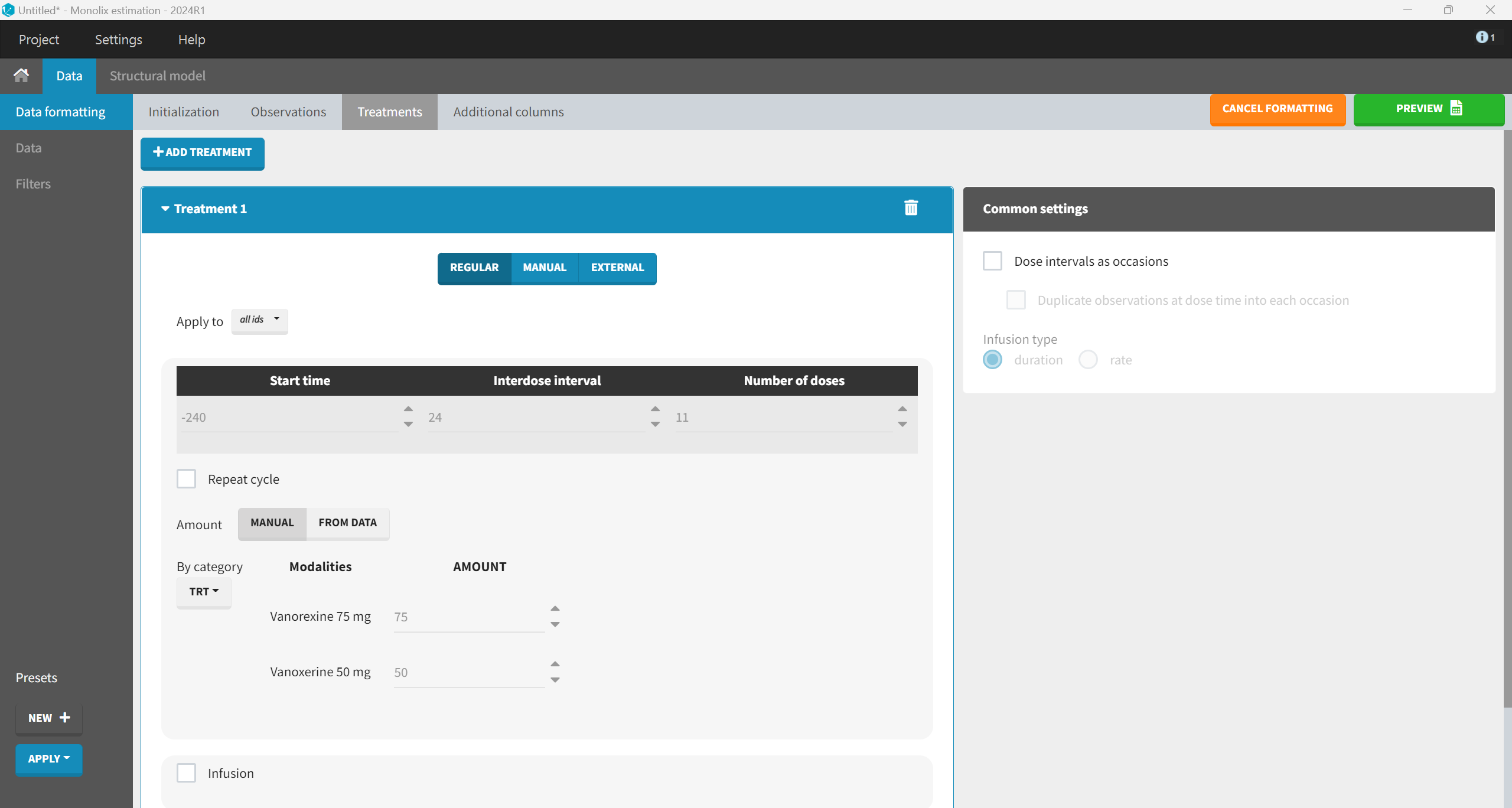
The drug administration information is added in the “Treatments” tab. An amount column is required to indicate the administered dose, where rows represent times of administration. It is created via the “+ Add treatment” option. The dataset does not contain any treatment administration information. It only provides data for Visit Day 11 with PK sampling at Time 0, 0.5, 1, 2, …, 12 hr. Therefore, treatment administrations must be added to feed the PK model.

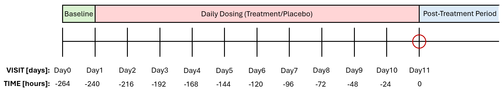
In the dataset, Visit Day 11 corresponds to TIME = 0 hours, where PK samples were collected. To stay consistent with the dataset’s TIME column, earlier dosing days (Days 1–10) must be represented by negative TIME values, counting back from Day 11. This way the full treatment schedule is aligned to the dataset’s time vector, and ensures that the PK model will take into account all doses.

Although the dosing schedule is defined in days in the study protocol, the dosing events must be created using hours to maintain consistency with the unit of the TIME variable in the dataset. Therefore, the start time should be set to -240 hours (corresponding to Day 1), with an interdose interval of 24 hours for the once-daily dosing regimen and 11 total doses to account for the complete dosing history prior to the final PK sampling day and the dose administered at Day 11. The amount information can be chosen manually based on the TRT column, which indicates the treatment group (Vanoxerine 50 mg or Vanoxerine 75 mg).

The “Preview” button shows that the additional rows and columns were created correctly. Before accepting the dataset, columns that were not automatically tagged must be manually tagged. In addition to SUBJID tagged as ID, TIME as TIME and the columns created by the data formatting AMT as AMOUNT, OBS as OBSERVATION and OBSID as OBSERVATION ID, we also tag TRT as CATEGORICAL COVARIATE (for plot stratification) and BLQTc_centAdjPl as CONTINUOUS COVARIATE (to be included as covariate in the model). When hiding the untagged columns, we obtain the following:

Pharmacokinetic (PK) model: Vanoxerine concentration

We will start by developing a model for the PK concentration first. Once data formatting is complete, the Observed Data Plot displays the PK data.

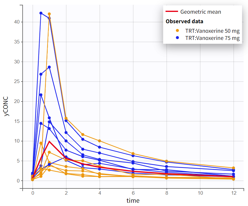
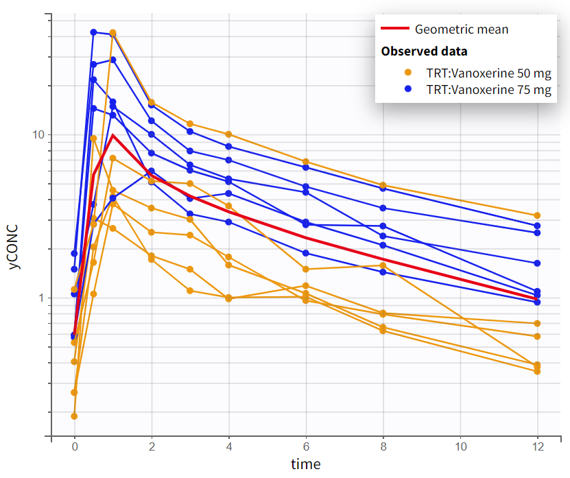
Exploratory data analysis

The observed data plot for the PK data provides an initial insight into the kinetics of vanoxerine after oral administration. On log-scale, the elimination phase shows a biphasic pattern, with two distinct linear slopes. This suggest that a 2-compartment model will be needed.

Observed PK data in linear scale	Observed PK data in semi-log scale

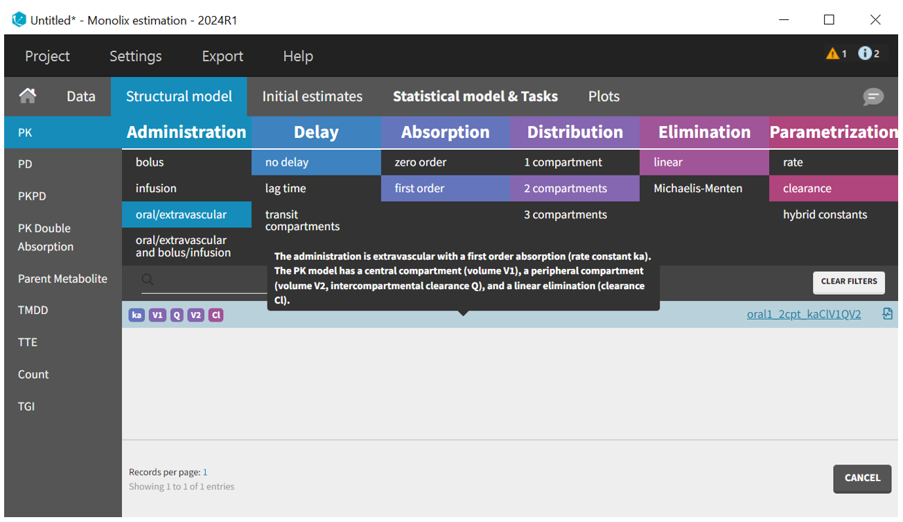
Structural PK model development

We start by defining the structural model. The built-in model libraries provides a large variety of models. The filters for the PK library, corresponding to the ADME processes, help to select a model from the list. We choose a model with “oral” administration, “no delay”, “first-order” absorption, “2 compartments” distribution (according to the data visualization), “linear” elimination and parametrized with “clearances”.

Once the structural model is selected, the Initial Estimates tab helps to find initial values for the estimation of population parameters. The auto-init function, which uses a custom optimization method on pooled data without inter-individual variability, very often provides good initial estimates.

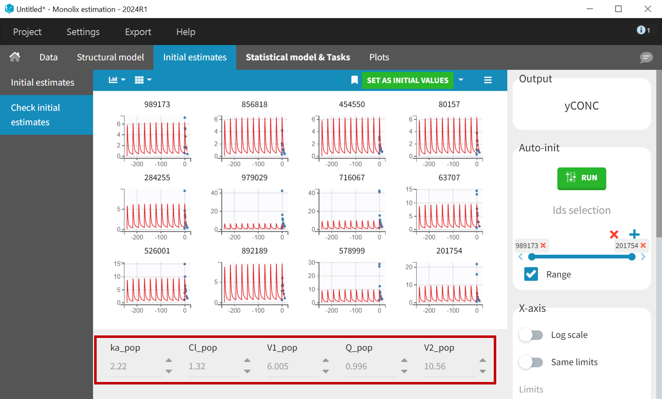
PK samples start at time = 0, so setting x-axis limits to helps to check weather the selected initial values capture the main characteristics of the profiles.

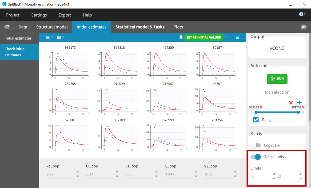
The button “Set as initial values” saves the new values as initial estimates for the population parameter estimation.

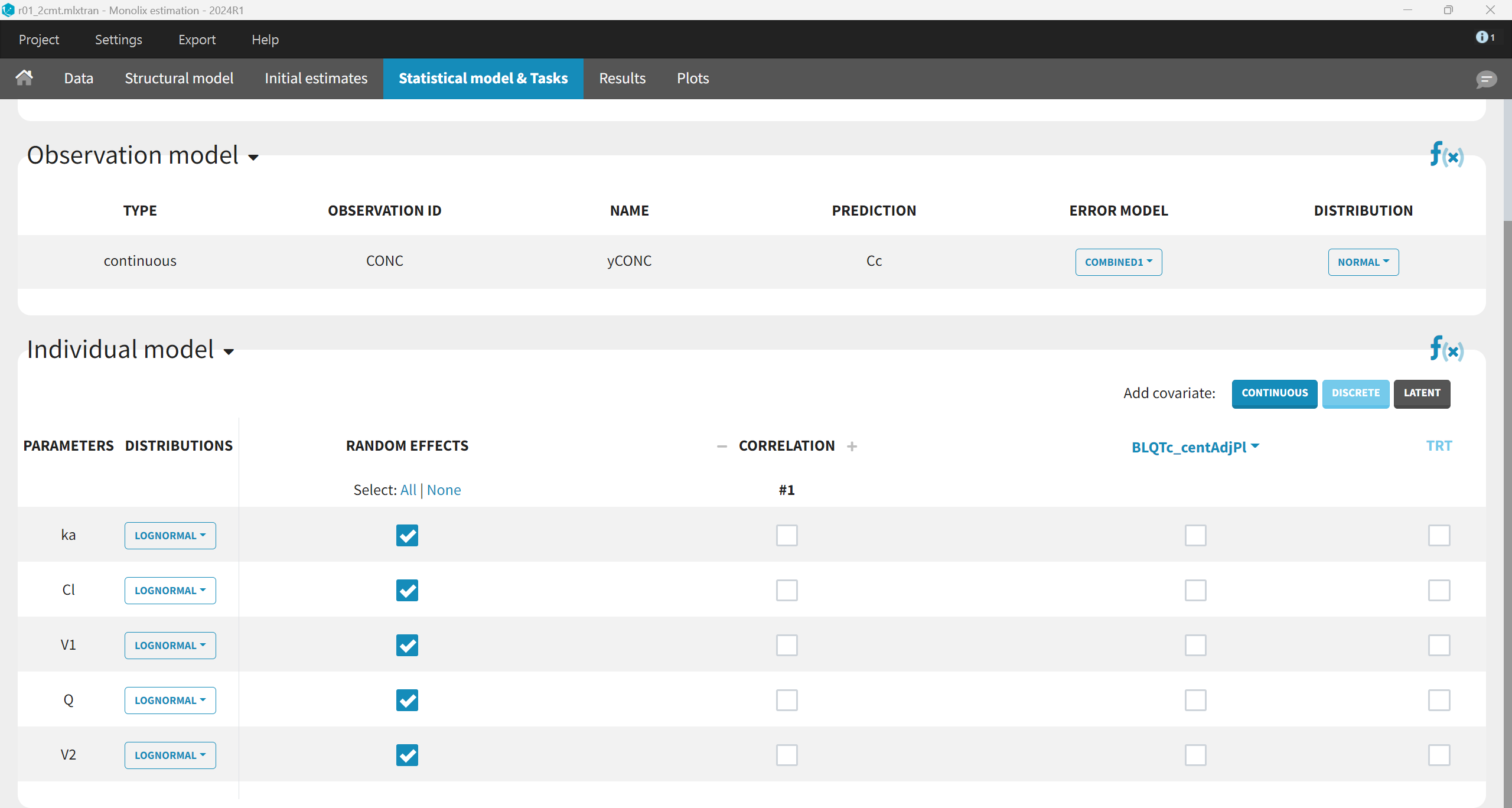
For the first run, we will use the default statistical model: “combined1” error model with a constant and a proportional error term, lognormal distribution for all parameters, inter-individual variability and no covariates for all parameters. In order to make sure have enough prediction time points to capture the 11 inter-dose intervals, the grid is changed to 10000 points in the Plots task settings. The project is saved as r01_2cmt.mlxtran and run including all estimation tasks with the option “use linearization method” for speed.

The results are the following:

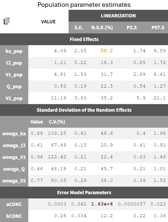
The error model parameter aCONC is estimated to be very small and highly uncertain (high RSE), indicating it may be removed by changing to a proportional error model. However, it is preferrable to change the error model after having worked on the structural model.

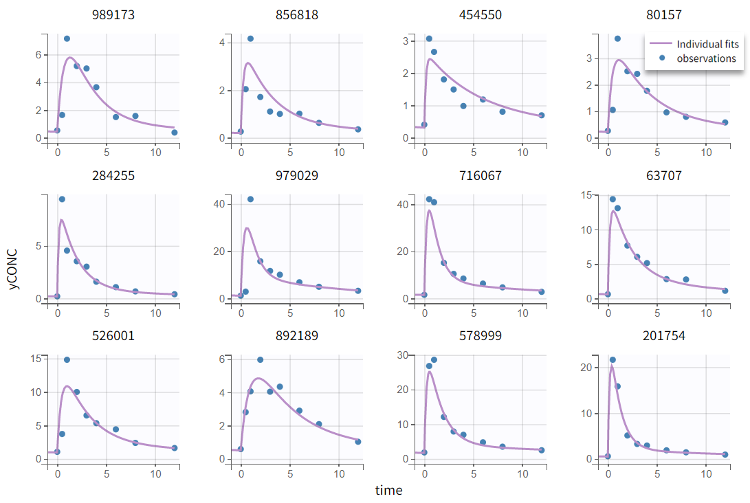
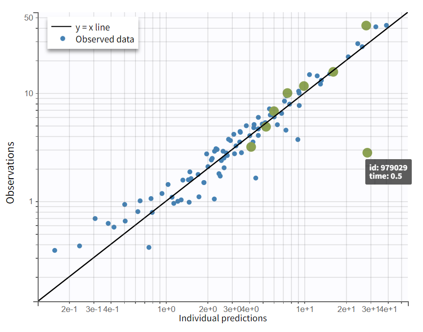
In the “Plots” tab, the individual fits (left) show that peak concentrations are underpredicted. Note that the axis limits can be adjusted to [-1, 12] in the Settings > Axes tab. In the observations vs. predictions plot (right), most points are well balanced around the unity line, with the exception of one early time point (time=0.5 hr) that lies well below the identity line, indicating overprediction in the absorption phase for individual 979029.

Individual fits	Observation vs predictions (log-log scale)

Overpredicted early time points and underpredicted peaks suggest a missing lag time. Adding a lag time parameter would shift the prediction curve to later time points and allow to steepen the absorption phase, improving the fit to peak concentrations. The next modeling step is therefore to include a lag time parameter in the structural model by choosing a new structural model with delay = “lag time” (lib:oral1_2cpt_TlagkaClV1QV2.txt).

In the “Initial estimates” tab, click “Use last estimates: Fixed effects” to use the final estimates of the previous run as initial values. The new parameter Tlag_pop should be set below 0.5 days, which is the time of the first measurement. Tlag_pop = 0.25 hours is appropriate. This new model is saved as r02_Tlag2cmt.mlxtran and run.

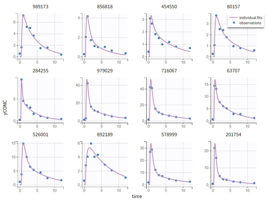
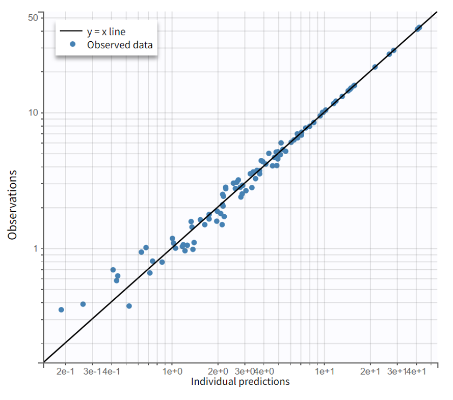
The resulting diagnostic plots show that including a lag time improves the fit, with observed data now captured more accurately than in the previous model.

Individual fits	Observation vs predictions (log-log scale)

Comparing the model run with first-order absorption and lag time to the previous run with first-order absorption only shows that the addition of a lag time not only improves the model fit visually, but also provides quantitative improvement.

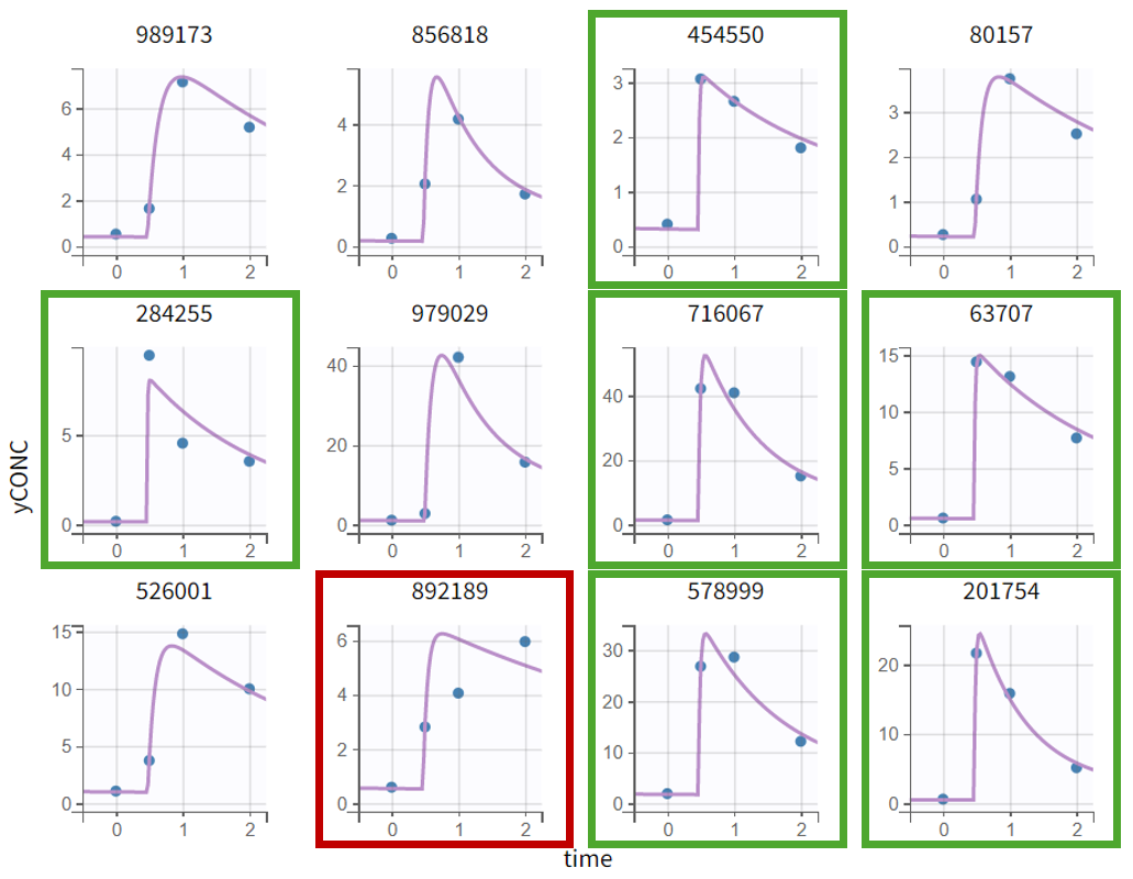
An examination of the final population estimates shows that some parameters now have high relative standard errors, in particular ka_pop (typical absorption rate) and omega_Tlag (between-subject variability in Tlag), and have thus a low confidence.

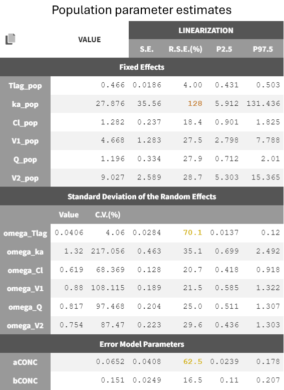
The high RSEs suggest challenges in accurately estimating the absorption process. With a lag time Tlag_pop = 0.466 h and a high absorption rate constant ka_pop = 27.9 /h, the model depicts a delayed onset followed by rapid absorption.

For the subjects highlighted in green below, no data points are available during the absorption phase. This leads to relatively long estimated lag times and a rapid concentration increase to match observed concentrations, contributing to the high ka_pop and its large uncertainty. About half of the individuals fall into this category, providing little information on absorption parameters. Thus, considering between-subject variability on both ka and Tlag might be too ambitious giving the data at hand. This will be explored in the next section.

Individual fits

Subject 892189 (red frame) shows a poor fit during absorption, suggesting that the first-order absorption model with lag time may not fully capture the process. Alternative models (zero-order, sigmoid absorption, transit compartments, weibull absorption) were explored, but given sparse absorption data for the vast majority of individuals, they could not be reliably supported.

For the remainder of the case study, the first-order absorption model with lag time (r02_Tlag2cmt.mlxtran) is retained as the most physiologically reasonable choice given the small number of subjects.

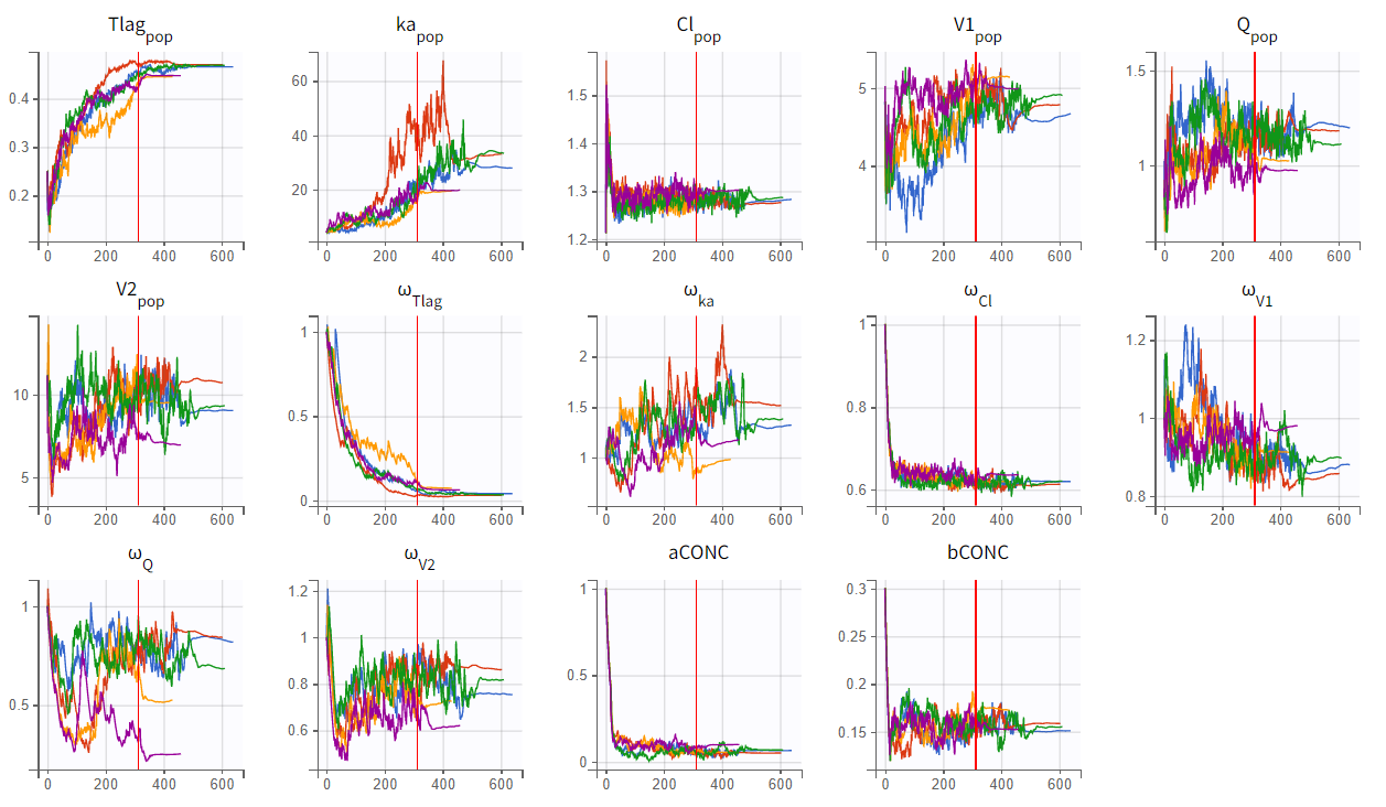
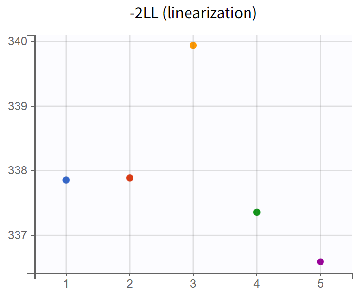
Assessment of parameter estimate robustness

To evaluate the stability of the run, a convergence assessment was performed by re-running the model five times with different seeds. Parameter estimates and likelihoods were consistent, with a maximum log-likelihood difference of about , indicating stable estimates. The model can therefore be considered a suitable structural model for further development.

Statistical PK model development

The statistical model consists of the residual error model and the individual model (parameter distribution, correlation between random effects and covariates).

Residual error model

The default combined 1 model resulted in a constant error parameter “a” with high uncertainty. The "Proposal" sub-tab in the "Results" section shows that all four available error models were tested in a preliminary fashion based on the current run information, and that the combined 2 model might provide the best fit according to the selection criteria. Compared to the combined 1 model, the combined 2 model has a slightly different formula.

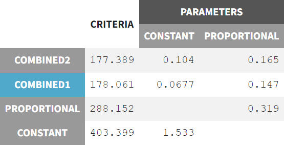
The model was rerun with the error model changed to combined 2 (r03_comb2Err.mlxtran) and initial values set to the last estimates from the fixed effect. The run yields the following estimates:

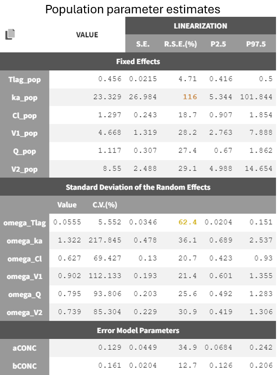
The new estimates show improved precision for the constant error term, with slightly reduced uncertainty in ka_pop and omega_Tlag. The BICc criteria indicate minimal differences between the combined 1 and combined 2 error models.

Nevertheless, the modification of the error model is considered beneficial, as it results in lower RSEs while maintaining similar goodness of fit values.

Individual model

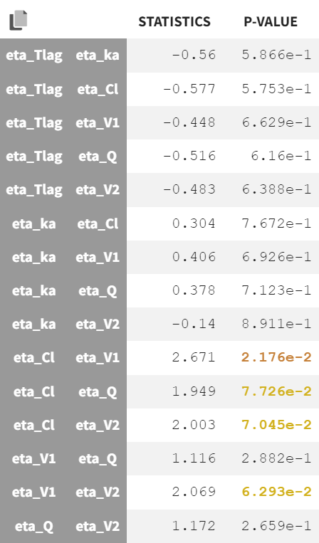
In the current run correlations were detected among random effects for Cl, V1, Q, and V2, as shown by scatterplots and significant correlation coefficients. These correlations can be included in the population model and be estimated.

Correlation between random effects

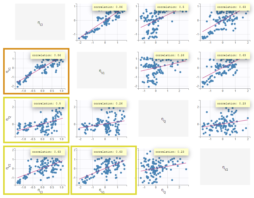
Correlations were added stepwise, starting with the strongest and re-estimating to assess improvements. Each correlation addition improves the likelihood. In the run r06_comb2Err_corrClV1QV, aCONC converged near zero with high uncertainty. Thus, the error model was simplified to a proportional error model. This leads to a worsening of the likelihood but an improvement of the BICc (due to the lower number of parameters), which justifies to keep the proportional error model.

The estimates of the run r07_propErr_corrClV1QV2 are shown below.

Six new population parameters were estimated, representing correlations among the random effects of Cl, V1, Q, and V2.

Most estimates were precise, while absorption-related parameters ka_pop and omega_Tlag still showed high uncertainty. The model can be simplified by removing the inter-individual variability on the absorption parameters. Removing the random effects on Tlag improves the BICc but leads to a worse RSE for ka_pop associated to a very high ka_pop estimate (174 /hr). Removing the random effects on ka leads to a worsening of the BICc. We thus decide to keep r07_propErr_corrClV1QV2 as final model.

A convergence assessment confirmed stable estimates with , within an acceptable range. The model can be considered sufficiently adequate to proceed with the QTc part of the analysis.

PKPD model: C-QTc interval relationship

Exploratory data analysis

The ΔΔQTc can be visualized similarly to the plots shown in the automatic QTc report presented above, and help to assess the shape of the conc-QTc relationship and the presence of a delay.

Observed data plot	Bivariate data viewer

The observed data plot displayed with respect to the concentration (Plot settings > Axes > Regressor Cc_reg on x-axis) shows the individual ΔΔQTc with respect to the concentration for all subjects. The trendline (mean calculated over 10 bins) suggests a saturating effect, which could be captured by an Emax model.

The bivariate plot shows the relationship between ΔΔQTc and drug concentration over time for each subject. Individual trajectories are visualized by connecting points in time order. Some individuals show a counterclockwise pattern, which can be the sign of a delay.

Model development

Given the hints for a saturating relationship and a delayed effect of the concentration on ΔΔQTc, we will test both the standard linear model and an Emax model, as well as models with direct effect or an effect compartment. We will first explain how to implement the linear model with direct effect, starting from the final PK run r07_propErr_corrClV1QV2.

Linear model

The standard linear model is:

To implement this model in Monolix, we will separate it into the structural model, which describes the relationship between the concentration and ΔΔQTc, and the statistical model, which describes the random effects and covariates effects (here the BLcentAdjPl variable).

The structural model thus reads:

while the statistical model reads:

The intercept parameter does not have a direct physiological interpretation but provides the model with flexibility to capture systematic differences between treatment and placebo. The slope parameter represents the strength of the drug effect on ΔΔQTc.

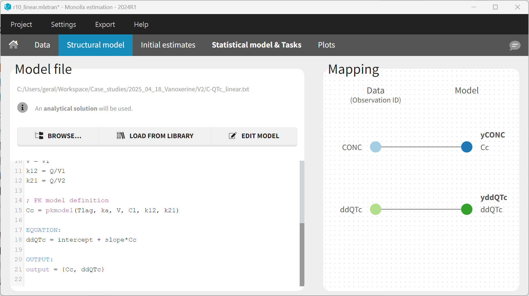
The structural model is defined using the mlxtran language, by appending the ΔΔQTc model to the PK model selected from the library, in the following way. This is done in the “Structural model” tab, after clicking on “Edit model”.

[LONGITUDINAL]
input = {Tlag, ka, Cl, V1, Q, V2, intercept, slope}


PK:
; Parameter transformations
V = V1
k12 = Q/V1
k21 = Q/V2

; PK model definition
Cc = pkmodel(Tlag, ka, V, Cl, k12, k21)


EQUATION:
ddQTc = intercept + slope * Cc


OUTPUT:
output = {Cc, ddQTc}

The input line defined the individual parameters which will be estimated. The PK part of the model is defined via the pkmodel() macro which calls the corresponding analytical solution in the background. The PD part is defined as a simple mathematical expression, which depends on the concentration Cc. Note that in the classical approach shown previously, the concentration is read from the dataset and used directly in the equation for the PD model. In the current joint PK/PD model, it is the model-predicted concentration which feeds into the PD model. This will be particularly important when using models with a delay. The output line defines the variables which will be mapped to the observations in the dataset.

After having edited the model, the “Mapping” panel allows to map the model output Cc to the observations with OBSID = CONC in the dataset, and the model output ddQTc to OBSID = ddQTc.

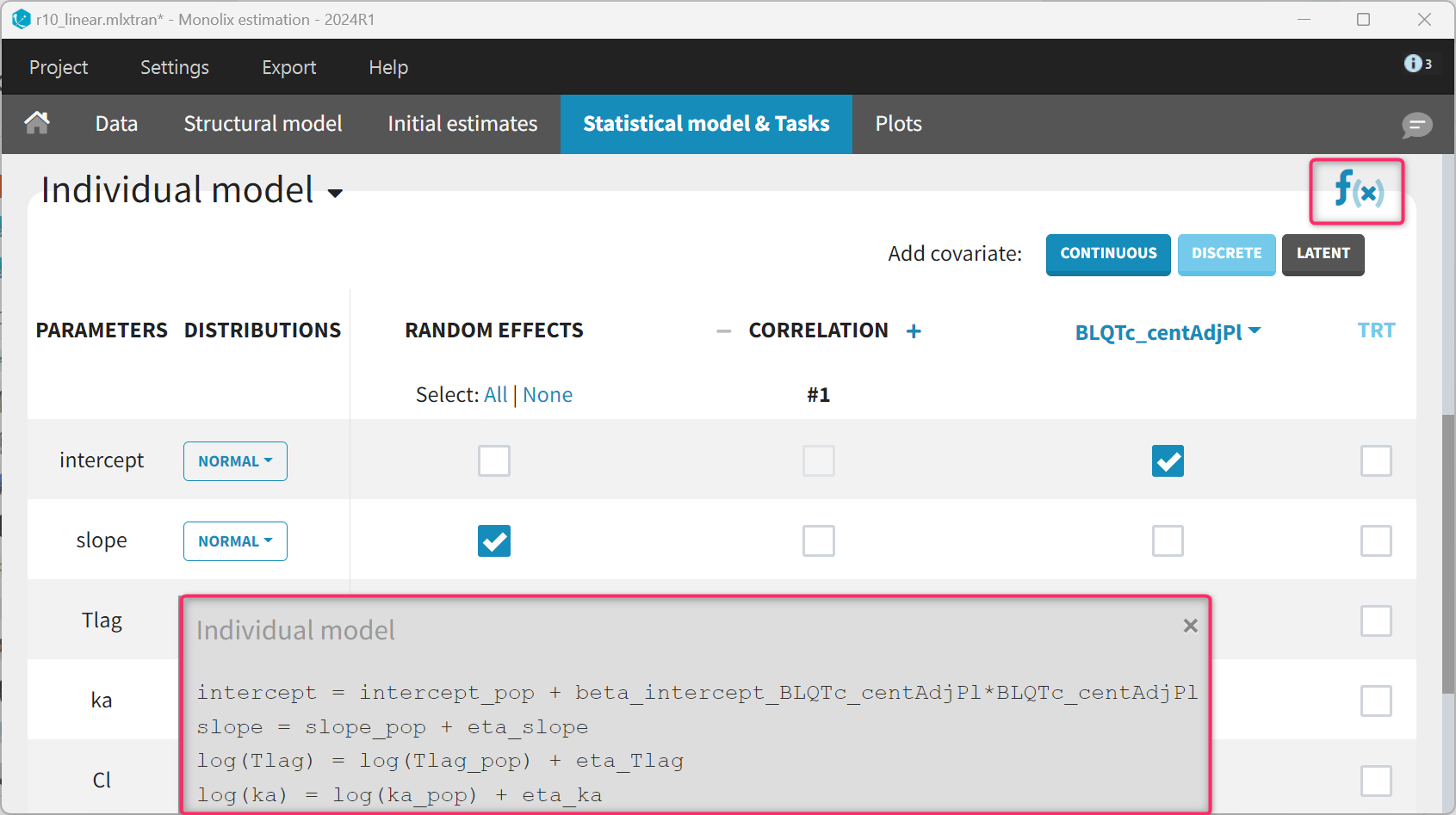
The statistical model for the PK part remains unchanged. For the ΔΔQTc model, the slope parameter is set to a normal distribution with random effects to mimic the standard model. For the intercept, the random effects are removed and the BLQTc_centAdjPl covariate is added. For the covariate to appear linearly in the model, the distribution of the intercept parameter must be set to “normal”. The corresponding equations can be displayed by clicking on the equation icon. Finally, the residual error model is set to “constant”.

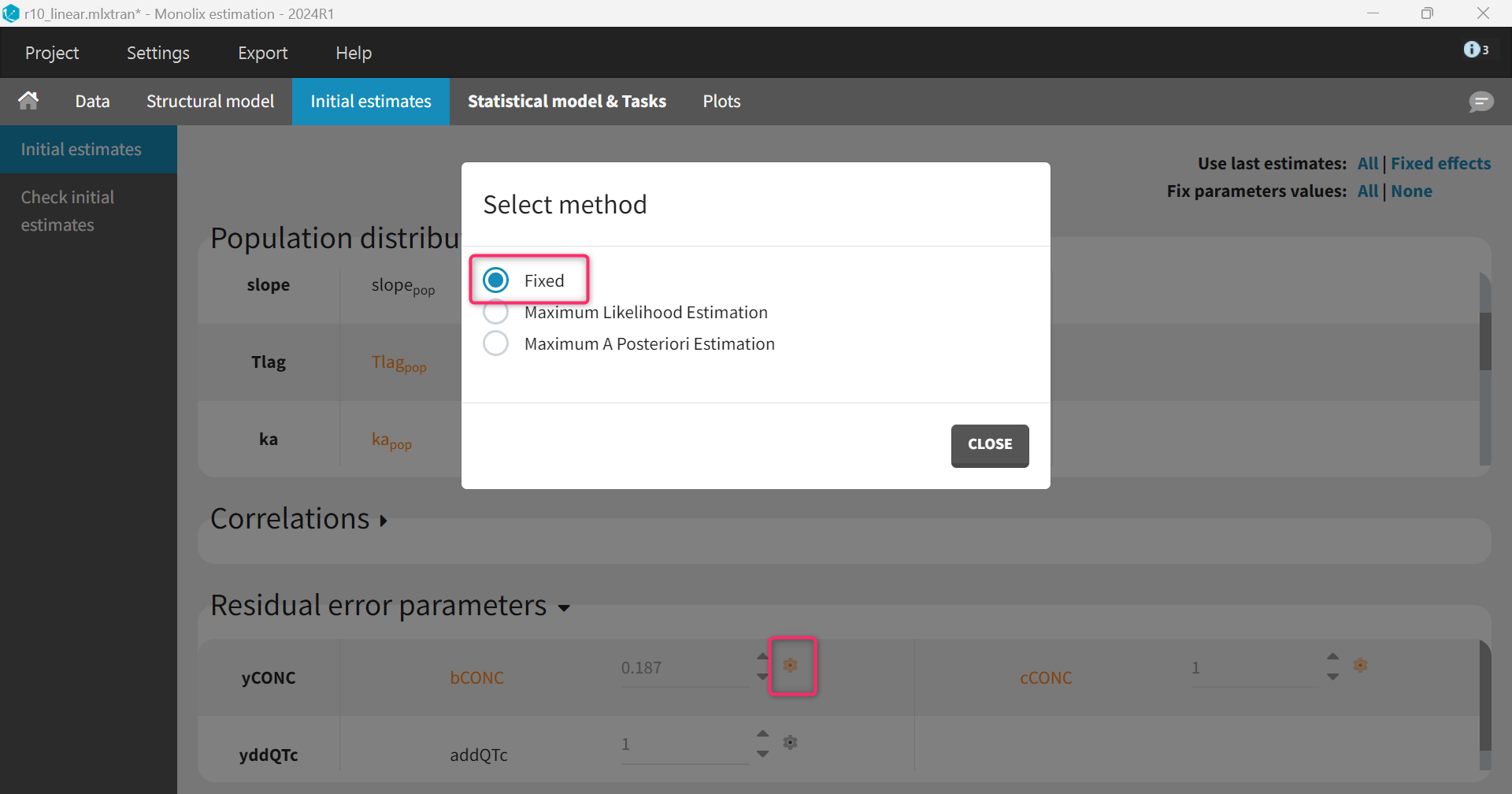
The parameters for the PK model have already been estimated and can be fixed to the estimates of the final PK run. This is done in the “Initial estimates” tab by clicking “Use last estimates: All” and then clicking on the wrench icon next to the parameters of the PK model and selecting “fixed”. Note that this can also be done before modifying the structural model, such that “Fix parameters values: All” can be selected to fix all PK parameters at once before adding the PD parameters.

Regarding the initial values of the PD model, intercept_pop is set to zero (its expected value). The slope_pop parameter has units L/mg (inverse of a concentration) and can be set to a value similar to the concentration typical value, in our case 10 (i.e assuming that a concentration of 10 mg/L leads to a 1 ms ΔΔQTc). The omega_slope parameter should be set equal to slope_pop to ensure a high initial inter-individual variability (IIV). Given that a normal distribution has been chosen, omega_slope = slope_pop corresponds to a 100% IIV.

Alternative models

Alternative models with saturating Emax instead of linear effect and delayed effect via an effect compartment will also be considered given the preliminary data exploration. These changes are will be applied in the structural model.

For the Emax model, the model equation can simply be modified to ddQTc = intercept + Emax * Cc/(Cc+EC50) and the input slope parameter replaced by Emax and EC50. For the statistical model, we keep random effects on the Emax parameter (similar to the slope previously) but remove them on EC50. Emax is set as “normal distribution” to allow for both positive and negative, while “lognormal distribution” is kept for EC50 which represents the concentration of half-maximum effect and is thus positive.

For the model with delay, the delay is captured via an effect compartment. The concentration in the effect compartment Ce can be defined via an ODE as ddt_Ce = (Cc - Ce)/tau with tau the characteristic time of the delay. However, the variable Ce can also be computed using an analytical solution as part of the pkmodel() macro, using the reserved keyword ke0, which is the inverse of the characteristic time tau. This allows faster runs and is done by extending the pkmodel() macro in the following way: {Cc, Ce} = pkmodel(Tlag, ka, V, Cl, k12, k21, ke0=1/tau). The additional parameter tau is assumed to be the same across individuals (i.e no random effects) with a lognormal distribution to remain positive.

The model with Emax effect and delay thus reads:

[LONGITUDINAL]
input = {Tlag, ka, Cl, V1, Q, V2, intercept, Emax, EC50, tau}


PK:
; Parameter transformations
V = V1
k12 = Q/V1
k21 = Q/V2

; PK model definition
{Cc, Ce} = pkmodel(Tlag, ka, V, Cl, k12, k21, ke0=1/tau)


EQUATION:
ddQTc = intercept + Emax*Ce/(Ce+EC50)


OUTPUT:
output = {Cc, ddQTc}

Model comparison

The four candidate models are run and compared in terms of BICc, which balances the likelihood and number of estimated parameters.

The best model (i.e lowest BICc) in the Emax model with delay, which is consistent with our previous exploratory data analysis.

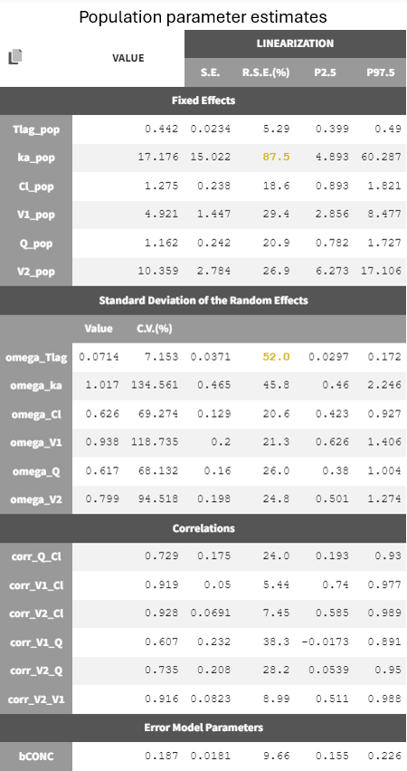
The estimated parameters and their RSEs are shown below. Some parameters have high RSEs indicating a high uncertainty in the parameter estimate. Simplifications of this model, e.g by removing random effects on Emax, could be explored. However, the Garnett et al white paper recommends to keep all terms in the model even if some are not well identifiable. This uncertainty will translate into the prediction interval obtained via simulations in the next step.

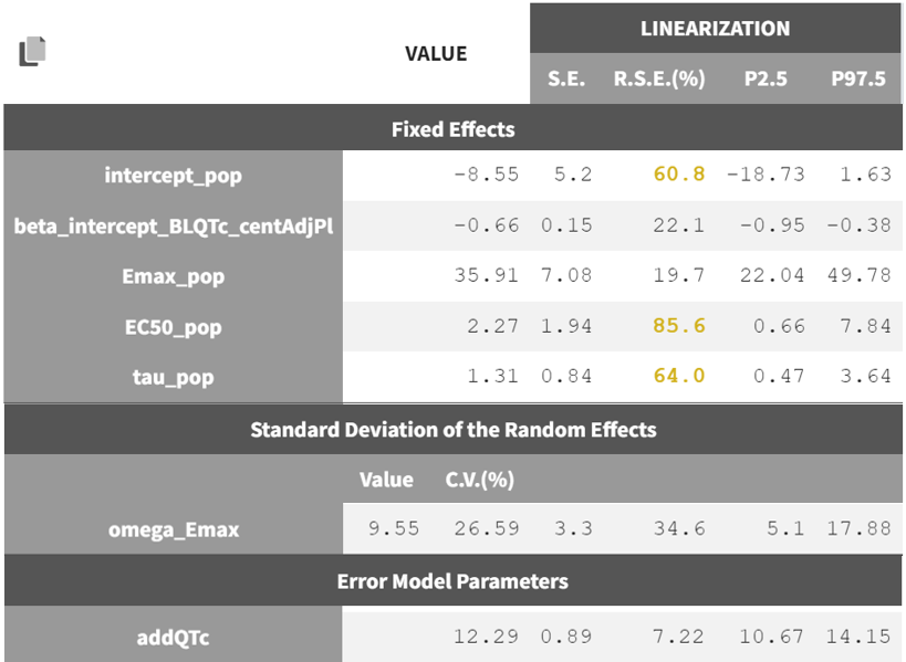
Note that the screenshot shown here only includes the PD parameters for clarity; the PK parameters remain unchanged as they are fixed. In the Monolix project, all model parameter estimates—both PK and PD—can be found under Results > Pop. param.

As a final step, the stability of the parameters estimates and likelihood can be confirmed via a convergence assessment. The consistent results over several replicates with different initial values prove a good model stability.

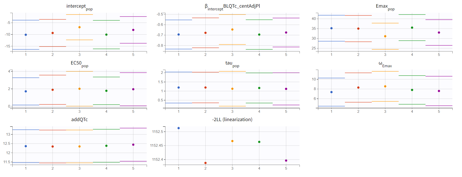
We thus consider the model with Emax concentration effect and delay as our final model.

Simulations

The simulations aim to assess whether the upper bound of the two-sided 90% confidence interval for the model-predicted ΔΔQTc remains below the regulatory threshold of 10 ms at concentrations of interest.

The usual procedure when working with a conc-QTc model is to define a range of concentrations and calculate the corresponding ΔΔQTc as ΔΔQTc = ϴ₁ + ϴ₂ * Cc (i.e using the intercept and concentration effect but ignoring the baseline effect). With a PK-QTc model, the model input is not a concentration anymore but the dosing regimen. For a given dosing regimen, the concentration and ΔΔQTc evolution can be predicted over time. Because of the delay, the time of maximum concentration and time of maximum ΔΔQTc will be different. To create (conc, ΔΔQTc) pairs for the plot, we will consider the maximum concentration and maximum ΔΔQTc over time for a large range of input dose levels.

The simulations will be conducted in Simulx via the lixoftConnectors R API.

The first step is to load the final Monolix project and export it to Simulx:

library(dplyr)
library(lixoftConnectors)
initializeLixoftConnectors(software="monolix", force=T)
library(ggplot2)

loadProject("r13_Emax_delay.mlxtran")
exportProject(settings=list(targetSoftware="simulx"), force=T)

The created Simulx project contains already several “elements” (for parameters, covariates, treatment regimens, and outputs) which can be used to define a simulation. And it is also possible to create new elements.

Using a notation similar to the Garnett et al paper, the PD part of our final model is:

To obtain the mean ΔΔQTc, we will consider a typical individual, i.e ignoring the random effects and the baseline effect (which is assumed to be null on average), and keeping only the fixed effects for the intercept and concentration effect. In Simulx, ignoring the random effect is easily done by using one of the population parameter elements starting with mlx_Typical. These elements contain the fixed effects as estimated in Monolix, and have omega parameters (i.e the standard deviation of the random effects) set to zero. To ignore the baseline effect, the easiest is to set the covariate BLQTc_centAdjPl to zero.

In addition, we need to compute the confidence interval of the prediction, which represents the uncertainty of the estimated fixed effects. When a linear model is used, an analytical formula is available. However, this formula cannot be generalized when non-linear models are used. An alternative would be to use non-parametric bootstrap, but this would require many runs. Instead, in Monolix, we can use the variance-covariance matrix of the estimates (from which the standard errors are derived and which is the inverse of the Fisher Information Matrix) to sample sets of (ϴ₁, ϴ_2, ϴ₅) parameters which capture their uncertainty, instead of using bootstrap replicates. Sampling sets of population parameters from their uncertainty distribution (still keeping omegas set to zero) is done very easily in Simulx by using the population parameter element mlx_TypicalUncertainLin and several replicates.

Finally, we need to define several dosing regimens, which will lead to several profiles for the concentration in plasma and the concentration in the effect compartment, which feeds into the ΔΔQTc model. We will reuse the same design as for the original dataset with a dose once a day for 10 days, but vary the dose amount in small increment from 0 to 100 mg. Each dose level will correspond to a different individual (with all individuals have the same individual parameters within a replicate, given that we ignore random effects).

For the simulation output, we will simulate the concentration in plasma and ΔΔQTc on a fine time grid for the last day, such that the maximum concentration and maximum ΔΔQTc can be extracted as a post-processing step.

The definition of the covariate, treatment and output is done via the defineXXXElement() functions. Each element is given a name which can then be used to set the element as part of the simulation scenario. The definition of the covariate and output element is done in the following way:

defineCovariateElement(name="covRef", element=data.frame(BLQTc_centAdjPl=0))

defineOutputElement(name="ddQTC_output", 
                    element = list(data=data.frame(start=0, interval=0.1, final=24), 
                                   output="ddQTc"))
defineOutputElement(name="Cc_output", 
                    element = list(data=data.frame(start=0, interval=0.1, final=24), 
                                   output="Cc"))

For the treatment element, we will consider 21 dose levels, from 0 to 100 mg by 5 mg increments. Each dose level correspond to a different individual, which id will be equal to the dose level. This information is formatted as a data.frame with columns id, time and amount. The data.frame cannot be given directly to simulx, but needs to be save as a csv file before.

doses <- seq(from=0, to=100, by=5) # mg
Nlevels <- length(doses)
times <- seq(from=-240, to=0, by=24) # time of doses
Ndoses <- length(times)
trt <- data.frame(id=rep(doses, each=Ndoses),
                  time=rep(times, Nlevels),
                  amount=rep(doses, each=Ndoses))

write.csv(trt, "treatment.csv", quote=T, row.names = F)

defineTreatmentElement(name="treatment", element=list(data="treatment.csv"))

The created elements are selected for the simulation using the setGroupElements() function, together with the element mlx_TypicalUncertainLin which was created during the export step. To sample population parameters from their uncertainty distribution, we need to set the number of replicates, here 200. For each replicate, we simulate a number of individuals equal to the number of dose levels (given that we have one individual per dose level).

setGroupElement(group="simulationGroup1", 
                elements=c("covRef", "treatment", "mlx_TypicalUncertainLin", "ddQTC_output", "Cc_output"))
setGroupSize(group="simulationGroup1", size=Nlevels)
setNbReplicates(200)

The simulation is launched with runSimulation() and the results retrieved with getSimulationResults(). We also rename the original_id column (which contains the id defined in the treatment element and were set equal to the dose level) to dose, to make the handling of the different dose levels clearer.

runSimulation()

ddQTc_pred <- getSimulationResults()$res$ddQTc %>% 
  mutate(dose = as.numeric(original_id))
Cc_pred <- getSimulationResults()$res$Cc %>% 
  mutate(dose = as.numeric(original_id))

For the ΔΔQTc, we calculate the maximum value over the time-profile for each dose and replicate. These values are then summarized as percentiles (5th, median and 95th) over the replicates. For the concentration, the simulations of all replicates are identical because the PK population parameters were fixed in the final Monolix run. We thus keep the simulations of the first replicate only and calculate the Cmax for each dose level. The concentration and ΔΔQTc data is then combined.

ddQTc_CI <- ddQTc_pred %>% 
  group_by(rep, dose) %>% 
  summarize(ddQTC_max=max(ddQTc)) %>% 
  ungroup() %>%
  group_by(dose) %>% 
  summarise(P5 = quantile(ddQTC_max, probs = 0.05, na.rm = TRUE),
            median = quantile(ddQTC_max, probs = 0.50, na.rm = TRUE),
            P95 = quantile(ddQTC_max, probs = 0.95, na.rm = TRUE)) %>% 
  ungroup()

Cc <- Cc_pred %>% 
  filter(rep==1) %>% 
  group_by(dose) %>% 
  summarize(Cc_max=max(Cc)) %>% 
  ungroup()

df <- cbind(Cc, ddQTc_CI[,-c(1)]) 

Two plots can be generated, using either the (maximum) concentration on the x-axis or the dose.

ggplot(df) + geom_ribbon(aes(x=Cc_max, ymin=P5, ymax=P95),fill='#00aedd', alpha=0.25) +
  geom_line(aes(x=Cc_max, y=median)) +
  xlab("Concentration (ng/mL)")+ theme_light() + ylab("ΔΔQTc (ms)") +
  geom_hline(yintercept = 10, linetype="dashed", size = 1, color = "black")+
  scale_x_continuous(breaks=seq(0,100,by=10))


ggplot(df) + geom_ribbon(aes(x=dose, ymin=P5, ymax=P95),fill='#00aedd', alpha=0.25) +
  geom_line(aes(x=dose, y=median)) +
  xlab("Dose (mg)")+ theme_light() + ylab("ΔΔQTc (ms)") +
  geom_hline(yintercept = 10, linetype="dashed", size = 1, color = "black") +
  scale_x_continuous(breaks=seq(0,100,by=10))

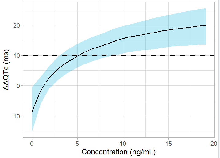
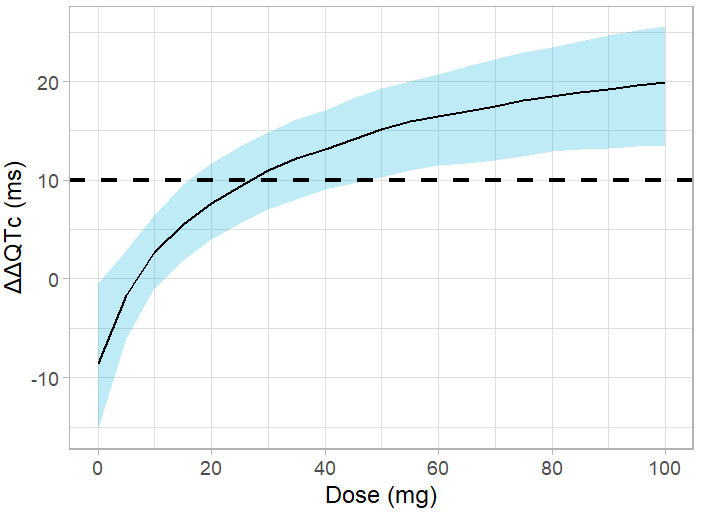
The upper bound of the confidence interval crosses the 10-ms threshold for a dose of 15 mg, corresponding to an average Cmax of 2.5 ng/mL. Thus, the planned dose of 50 or 75 mg bears a risk of significant QT interval prolongation.

Conclusion

A conc-QTc modeling approach was applied to a phase I study of Vanoxerine in cocaine-experienced volunteers. The standard approach was first implemented using the conc-QTc R package which allows to format the data, generate conc-ΔQTc models and produce a report with all standard exploratory and diagnostic plots.

In order apply the pre-specified linear model, the following assumptions must be fulfilled: (1) No drug effect on HR, (2) QTc interval is independent of HR, (3) No time delay between drug concentrations and ΔQTc or ΔΔQTc and (4) Linear C-QTc relationship. For Vanoxerine, the data exploration analysis presented in the report showed the presence of a time delay and a saturating conc-QTc relationship. When a delay is detected, the time of maximum concentration may be substantially different from the time of maximum effect. It is thus necessary to develop a population PK/QTc model, that models not only the effect of concentration on QTc, but also the shape of the concentration over time.

We proceeded with a stepwise PK/ΔQTc model development, starting with the PK data followed by the ΔQTc. The PK data was well captured by a 2-compartment model with first-order absorption and a lag time. To capture the conc-ΔQTc relationship adequately, it was necessary to introduce an effect compartment to create a delay, and consider an Emax relationship between the concentration in the effect compartment and ΔQTc.

The PK/ΔQTc model was then used to simulate the model-predicted ΔΔQTc and its 90% confidence interval. This step deserves particular care given the lack of a direct relationship between the concentration and ΔQTc. The upper bound of the confidence interval crosses the 10-ms threshold for a dose of 15 mg, corresponding to an average Cmax of 2.5 ng/mL.

The development of Vanoxerine was interrupted at Phase II because patients under treatment showed prolongation of the QT interval.

This example demonstrates a robust conc-QTc analysis workflow in the case where a delay has been detected and the pre-specified model cannot be applied. The publicly available R scripts can serve as a template for the analysis of other drugs.