Observation model (residual error)

For continuous data, the observation model is the link between the prediction f of the structural model and the observation. Thus, the observational model is an error model representing the noise and the uncertainty of the measurements. In Monolix, the observation model can be defined only in the interface.

Introduction

For continuous data, we are going to consider scalar outcomes () and assume the following general model:

for i from 1 to N, and j from 1 to , where is the parameter vector of the structural model f for individual i. The residual error model is defined by the function g which depends on some additional vector of parameters ξ. The residual errors are standardized Gaussian random variables (mean 0 and standard deviation 1). In this case, and are the conditional mean and standard deviation of , i.e.,

Available observation models

Residual errors

In Monolix, we only consider the function g to be a function of the structural model f, i.e.  leading to an expression of the observation model of the form

The following error models are available in the interface of Monolix and as model keywords in Simulx:

• constant: . The function g is constant, and the additional parameter is .

• proportional: . The function g is proportional to the structural model f, and the additional parameters are . By default, the parameter c is fixed at 1 and  the additional parameter is .

• combined1: . The function g is a linear combination of a constant term and a term proportional to the structural model f, and the additional parameters are (by default, the parameter c is fixed at 1).

• combined2: . The function g is a combination of a constant term and a term proportional to the structural model f(g = bf^c), and the additional parameters are (by default, the parameter c is fixed at 1). It is equivalent to where e1 and e2 are sequences of independent random variables normally distributed with mean 0 and variance 1.

Notice that the parameter c is fixed to 1 by default. However, it can be unfixed and estimated.

It is also possible to assume that the residual errors are correlated.

Positive gain on the error model
The second parameter b in the observational models comb1 and comb1c can be forced to be always positive by selecting b>0.

Distributions

The assumption that the distribution of any observation is symmetrical around its predicted value is a very strong one. If this assumption does not hold, we may want to transform the data to make it more symmetric around its (transformed) predicted value. In other cases, constraints on the values that observations can take may also lead us to transform the data.

The model extended model with a transformation of the data is then :

As we can see, both the data  and the structural model f are transformed by the function u so that remains the prediction of . Classical distributions are proposed as transformation:

• normal: u(y) = y. This is equivalent to no transformation.

• lognormal: u(y) = log(y). Thus, for a combined error model for example, the corresponding observation model writes . It assumes that all observations are strictly positive. Otherwise, an error message is thrown. In case of censored data with a limit, the limit has to be strictly positive too. [Note: if your observations are already log-transformed in your dataset, then you should not use that distribution as y in the formula would correspond to log-transformed measurements. Instead use the normal distribution.]

• logitnormal: u(y) = log(y/(1-y)). Thus, for a combined error model for example, corresponding observation model writes . It assumes that all observations are strictly between 0 and 1. However, we can modify these bounds to define the logit function between a minimum and a maximum, and the function u becomes u(y) = log((y-y_min)/(y_max-y)). Again, in case of censored data with a limit, the limits has to be strictly in the proposed interval too.

Combinations of distribution and residual error model

Hence, the following observation models can be defined with a combination of distribution and residual error model:

• exponential error model: and → constant error model and a lognormal distribution.

• logit error model → constant error model and a logitnormal distribution.

• band(0,10): → constant error model and a logitnormal distribution with min and max at 0 and 10 respectively.

• band(0,100): → constant error model and a logitnormal distribution with min and max at 0 and 10 respectively.

Defining the residual error model from the Monolix GUI

A menu in the frame Statistical model & Tasks of the main GUI allows one to select both the error model and the distribution as on the following figure (in blue and green respectively)

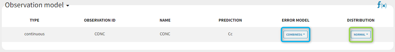
with the available options:

• Error model: combined1, combined2, constant, proportional.

• Distribution: normal, lognormal, logitnormal. For logitnormal, min and max values can be defined.

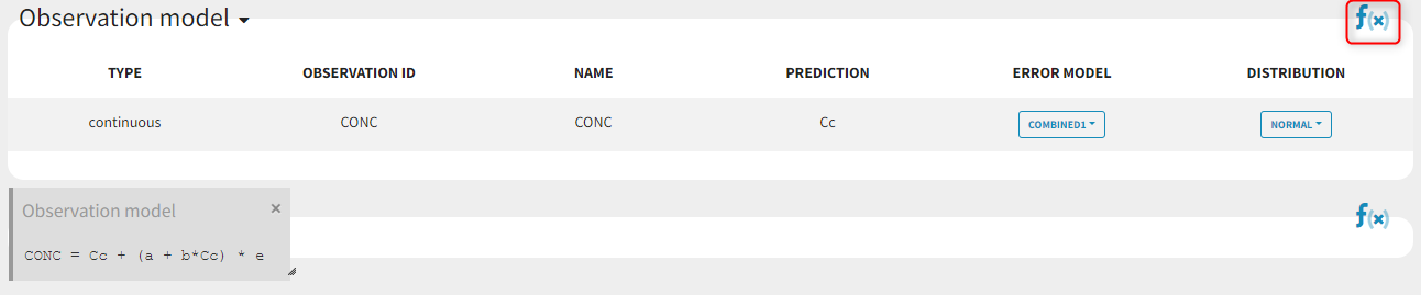
Any questions on what is the formula behind your observation model? There is a button in the interface as on the figure below where the observation model is described linking the observation (named CONC in that case) and the prediction (named Cc in that case). Note that ϵ is noted e here.

Some basic residual error models

• warfarinPK_project (data = ‘warfarin_data.txt’, model = ‘lib:oral1_1cpt_TlagkaVCl.txt’)

The residual error model used with this project for fitting the PK of warfarin is a combined error model, i.e. .

Several diagnosis plots can then be used for evaluating the error model. The observation versus prediction figure below seems ok.

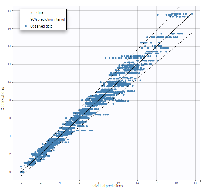
Remarks:

• Figures showing the shape of the prediction interval for each observation model available in Monolix are displayed here.

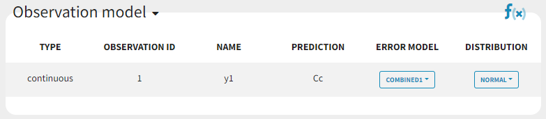
• When the residual error model is defined in the GUI, a bloc DEFINITION: is then automatically added to the project file in the section [LONGITUDINAL] of <MODEL> when the project is saved:

DEFINITION:
y1 = {distribution=normal, prediction=Cc, errorModel=combined1(a,b)}

Residual error models for bounded data

• bandModel_project (data = ‘bandModel_data.txt’, model = ‘lib:immed_Emax_null.txt’)

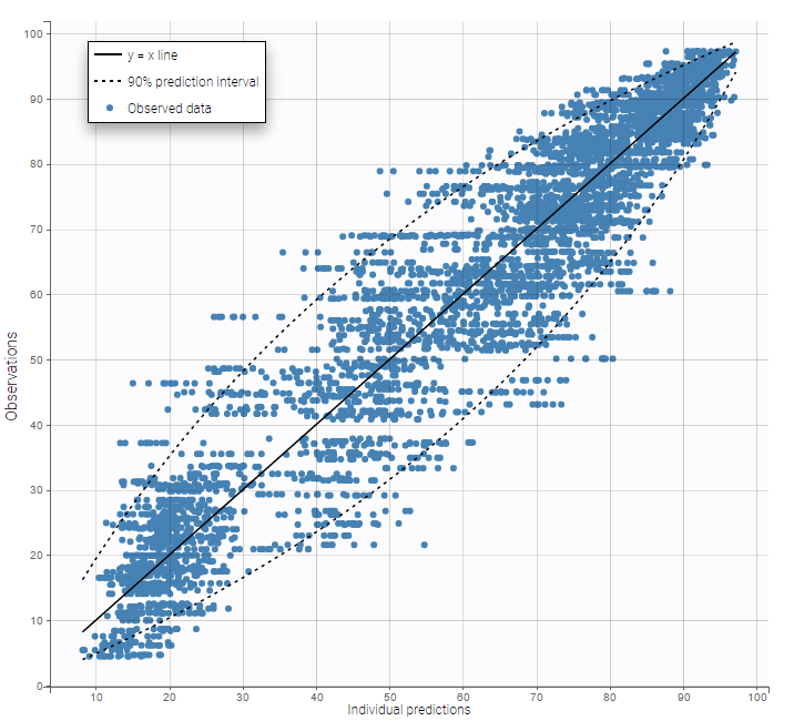
In this example, data are known to take their values between 0 and 100. We can use a constant error model and a logitnormal for the transformation with bounds (0,100) if we want to take this constraint into account.

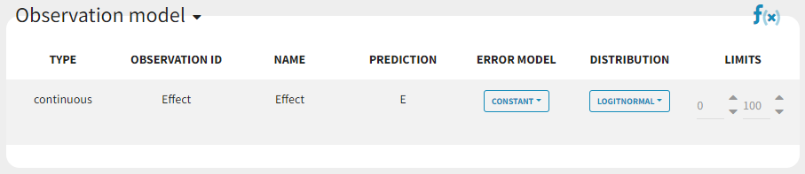
In the Observation versus prediction plot, one can see that the error is smaller when the observations are close to 0 and 100 which is normal. To see the relevance of the predictions, one can look at the 90% prediction interval. Using a logitnormal distribution, we have a very different shape of this prediction interval to take that specificity into account.

VPCs obtained with this error model do not show any mispecification:

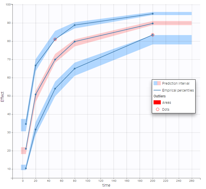
This residual error model is implemented in Mlxtran as follows:

DEFINITION:
effect = {distribution=logitnormal, min=0, max=100, prediction=E, errorModel=constant(a)}

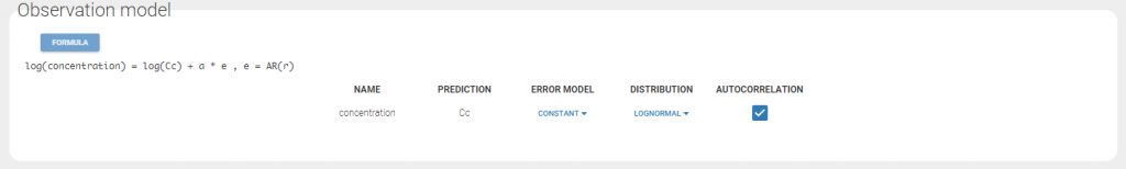
Autocorrelated residuals

Starting from version 2023R1, autocorrelation is not available in the interface when creating new projects. However, projects created with older versions that contain autocorrelation can still be opened. To use autocorrelation with new projects, the user should either use the connectors, or write it directly in the Mlxtran file:

• add “autoCorrCoef=r” in definition “DV = {distribution=normal, prediction=Cc, errorModel=proportional(b), autoCorrCoef=r}”, for example

• add “r” as an input parameter.

For any subject i, the residual errors are usually assumed to be independent random variables. The extension to autocorrelated errors is possible by assuming, that is a stationary autoregressive process of order 1, AR(1), which autocorrelation decreases exponentially:

where for each individual i. If for any (i,j), then and the autocorrelation function for individual i is given by

The residual errors are uncorrelated when .

• autocorrelation_project (data = ‘autocorrelation_data.txt’, model = ‘lib:infusion_1cpt_Vk.txt’)

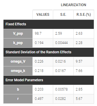
Autocorrelation is estimated since the checkbox r is ticked in this project:

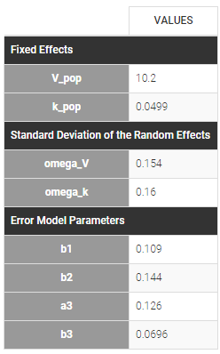
Estimated population parameters now include the autocorrelation r:

Important remarks:

• Monolix accepts both regular and irregular time grids.

• For a proper estimation of the autocorrelation structure of the residual errors, rich data is required (i.e. a large number of time points per individual) .

Using different error models per group/study

• errorGroup_project (data = ‘errorGroup_data.txt’, model = ‘errorGroup_model.txt’)

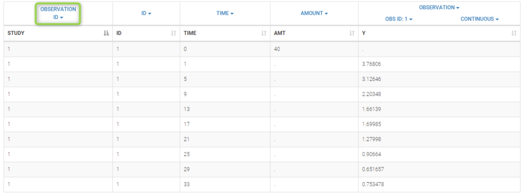
Data comes from 3 different studies in this example. We want to have the same structural model but use
different error models for the 3 studies. A solution consists in defining the column STUDY with the reserved keyword OBSERVATION ID. It will then be possible to define one error model per outcome:

Here, we use the same PK model for the 3 studies:

[LONGITUDINAL]
input = {V, k}

PK:
Cc1 = pkmodel(V, k)
Cc2 = Cc1
Cc3 = Cc1

OUTPUT:
output = {Cc1, Cc2, Cc3}

Since 3 outputs are defined in the structural model, one can now define 3 error models in the GUI:

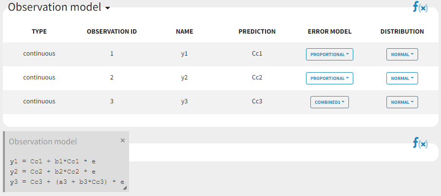
Different residual error parameters are estimated for the 3 studies. One can remark than, even if 2 proportional error models are used for the 2 first studies, different parameters b1 and b2 are estimated: