A simple TTE model for the Veterans’ Administration Lung Cancer study

Download data set only | Download Monolix project files

This case study presents a comprehensive modeling and simulation workflow on a time-to-event (TTE) dataset. It is recommended to first review the Introduction to TTE data and library of models in Monolix.

A second case study on time-to-event data is also available: Case study on NCCTG lung cancer data set

In this case study, a model is developed for the survival of patients with advanced lung cancer. It demonstrates how to evaluate the effect of various covariates, including a novel chemotherapy, and then applies the final model to simulate new scenarios.

• Introduction

• Data set visualization

• Population modelling in Monolix

  • Structural model

  • Covariate search

• Simulations in Simulx

  • Simulations using lixoftConnectors

  • Simulations using RsSimulx function

• Conclusion

Introduction

The following study has been conducted by the US Veterans Administration. It contains male patients with advanced inoperable lung cancer who received either a standard therapy or a test chemotherapy. Time to death was recorded for 137 patients, while 9 left the study before death. The study includes also various covariates for each patient.
The primary goal is to assess if the test chemotherapy is beneficial. Secondary goals include the analysis of covariates as prognostic variables.
This data set has been initially presented and analyzed in:

D Kalbfleisch and RL Prentice (1980), The Statistical Analysis of Failure Time Data. Wiley, New York.

Data set visualization

The data set includes data for 137 patients, 9 of them are right censored. According to the data set formatting guidelines, the data set includes for each patient a line indicating the start time (time = 0 and observation Y = 0), and a line indicating either the time of death (Y = 1) or the time at which the patient has left the study (Y = 0).
In addition the following covariates were recorded:

• Treatment (“trt” column): “standard” or “test” (tested new chemotherapy)

• Histological type of the tumor (“celltype” column): “squamous”, “smallcell”, “adeno” or “large”

• Karnofsky score (“karno” column): performance score that describes the overall patients status at the beginning of the study. The scale goes from 0 (dead) to 100 (completely healthy). More details about the scale can be found here.

• Time between diagnosis and start of the study (column “diagtime”): in months

• Age (column “age”): in years

• Prior therapy (column “priortherapy”): indicates if the patient has received another therapy before the current one

A snapshot of the data set in shown below:

We start with a visualization of the data set in Monolix: open Monolix, click on New project and Browse the data set. The figure below show the columns tagging (the covariates must be assigned to CONTINUOUS COVARIATE for continuous covariates or CATEGORICAL COVARIATE for categorical covariates):

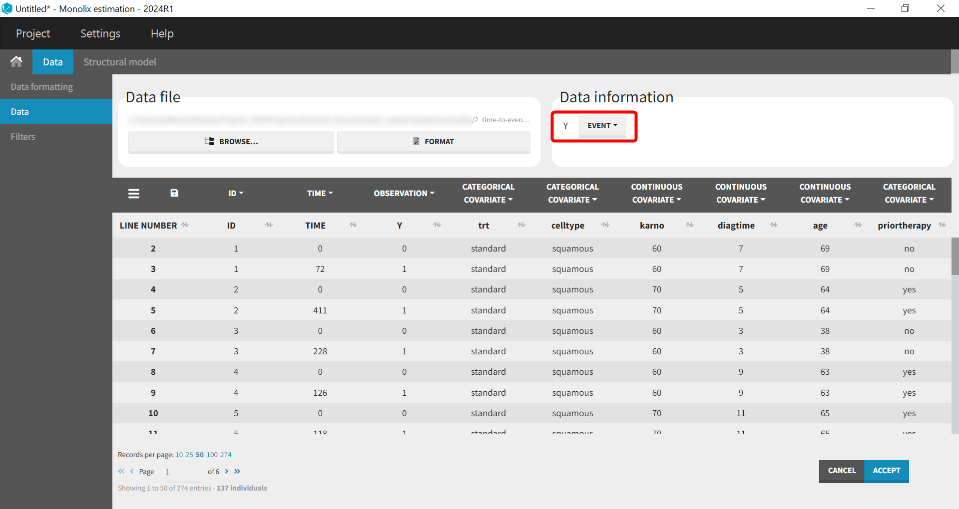
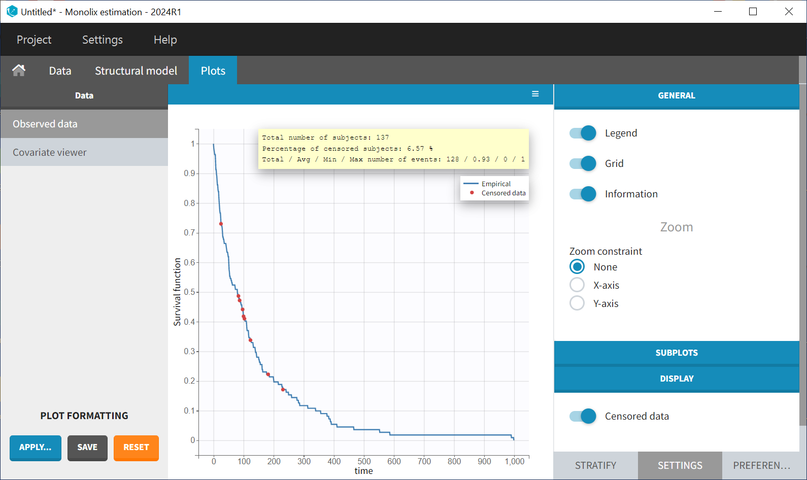
Before “Accepting” the dataset, we must indicate that the data is of type TTE (rather than continuous) – “Data information” section Y:EVENT. We can now accept the column assignments by clicking on “ACCEPT” button. A new tab “Plots” appear, where we can visualized the TTE data: the Kaplan-Meier (KM) estimate of the survival curve and the mean number of events curve (SUBPLOTS). Censored data are marked in red in the KM survival curve, and can be removed from the DISPLAY settings.

In the Stratification panel, the Kaplan-Meier curve can be split according to categorical or continuous covariates (or stratification covariates) and then "merged " into one figure, with each curve displayed in fixed colors. The legend provides information on the color assignment. Stratifying by the treatment variable "trt" (and using the "merge" option) results in the following figure:

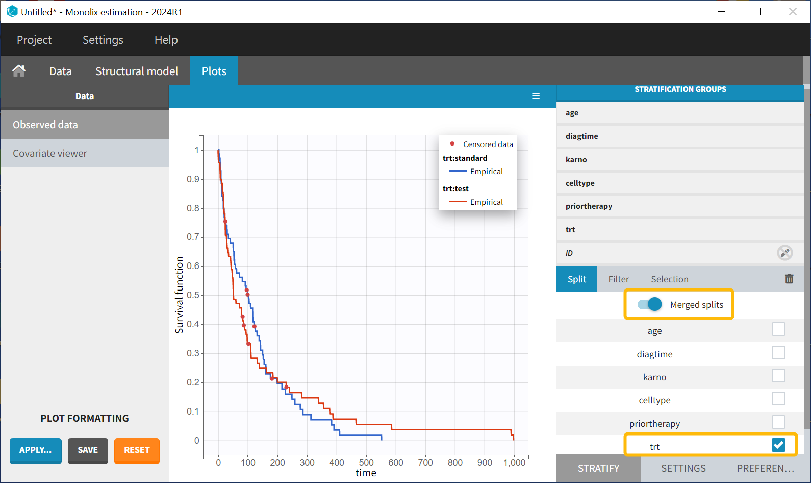
There appears to be no noticeable difference in survival between the standard treatment group and the chemotherapy treatment group based on the plot. Stratification using the Karnofsky score in two groups (Group1 = karno<50, and Group2 = karno>50) gives:

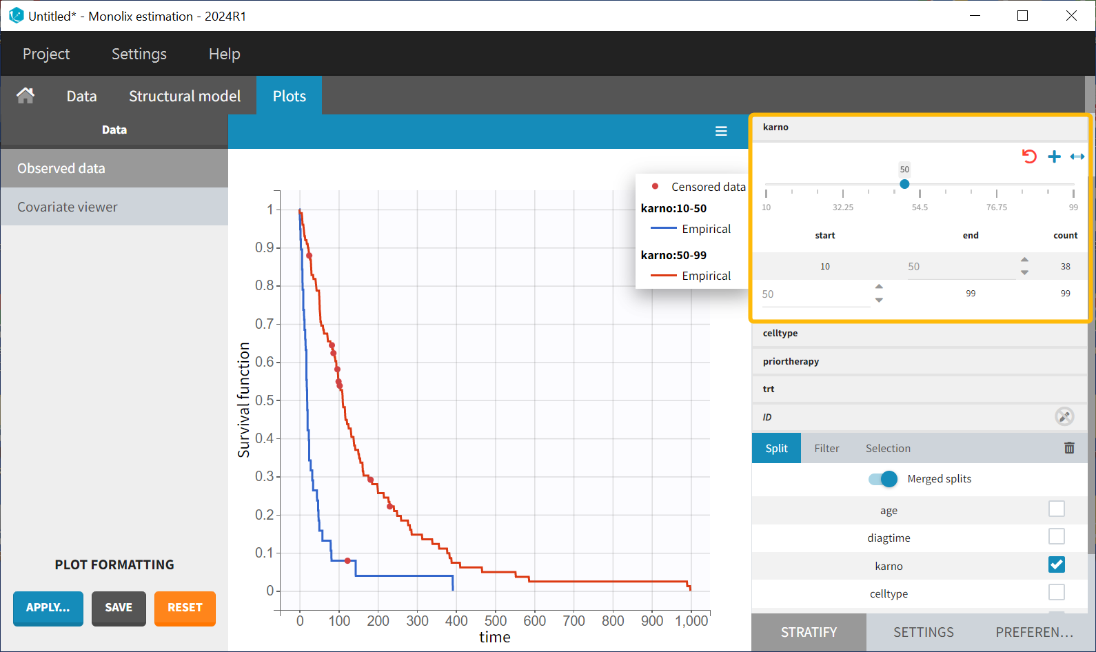
It is observed that patients with a higher Karnofsky score (indicating better overall health) tend to have longer survival. The tumor's histological type, “celltype,” also influences the survival curve. Squamous and large cell types appear to be less malignant, as patients with these types tend to survive longer.

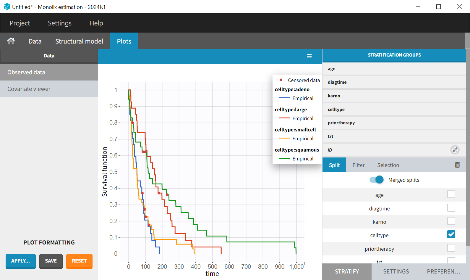
Note also that the survival curves for “adeno” and “small cell” types are very similar, so for comparison, these two groups could be joined together (drag&drop method in the stratification group).

Population modelling in Monolix

The next step is to develop a model for this data set and analyze the influence of covariates, particularly the treatment. In the MonolixSuite, the model must be fully defined through its hazard function, as non-parametric or semi-parametric approaches are not supported.

Structural model

The first step is to specify the structural model. The TTE introduction provides an overview of the library of common TTE models (defined via their hazard functions) and a presentation of the typical shapes of the resulting survival curves. Based on the data visualization, the Kaplan-Meier curve and the model library overview in the TTE introduction, the exponential model appears to be the most suitable choice. Therefore, the model file “exponential_model_singleEvent.txt” is selected from the library, with a single event type since death occurs only once per individual.

Next, the distribution of the individual parameters is defined.

• Most of the time in survival analysis, one assumes that the individual parameters are influenced by the covariates and all individuals with the same covariates have the same individual parameters – thus the same hazard function (but different times of death).

• Alternatively, a random effect can be assumed for individual parameters (often referred to as frailty models), which captures variability between individuals that cannot be explained by covariates.

Monolix’s estimation algorithms and plots are most effective when parameters include random effects, so this approach is used.

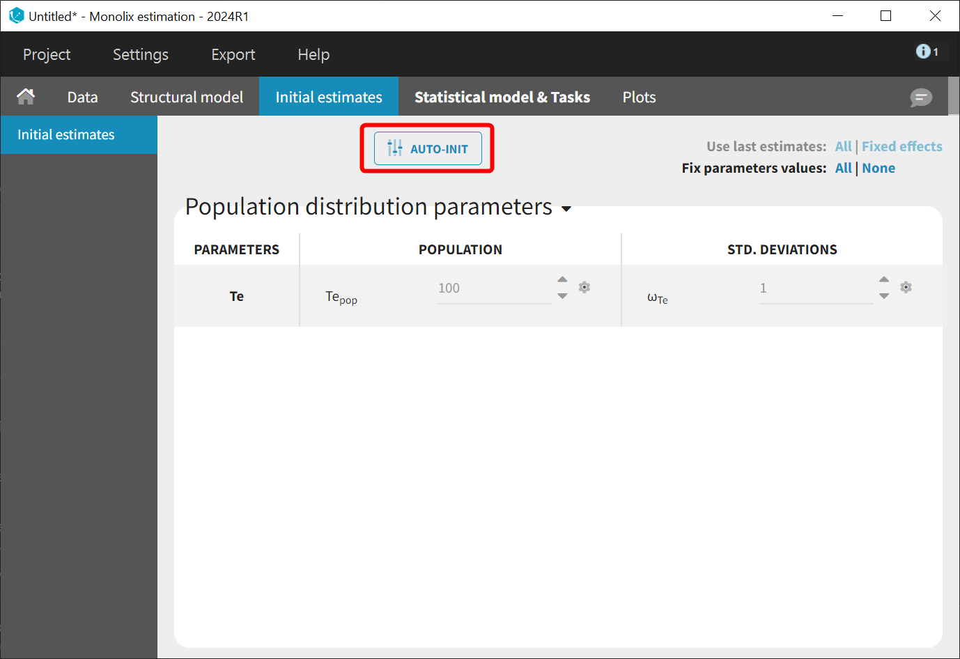
The model contains a single parameter, the characteristic time Te​, which should remain positive. Therefore, the default log-normal distribution is assumed. An initial value for this parameter can be chosen using the library overview—100, for example, for this data set. Starting from the 2021R1 version of MonolixSuite, AUTO-INIT is also available for time-to-event models.

Once the model is defined, the estimation tasks can be executed. This includes estimating the population parameters, calculating the standard errors using the Fisher Information Matrix, estimating the log-likelihood, and generating the relevant plots (note that individual parameters are skipped since individual fit plots are not possible with TTE data). The parameter Te​ rapidly converges toward a random walk around the maximum likelihood estimate (MLE) during the exploratory phase of SAEM (before the red line, as shown in the figure below), and then fully converges to the MLE during the smoothing phase (after the red line).

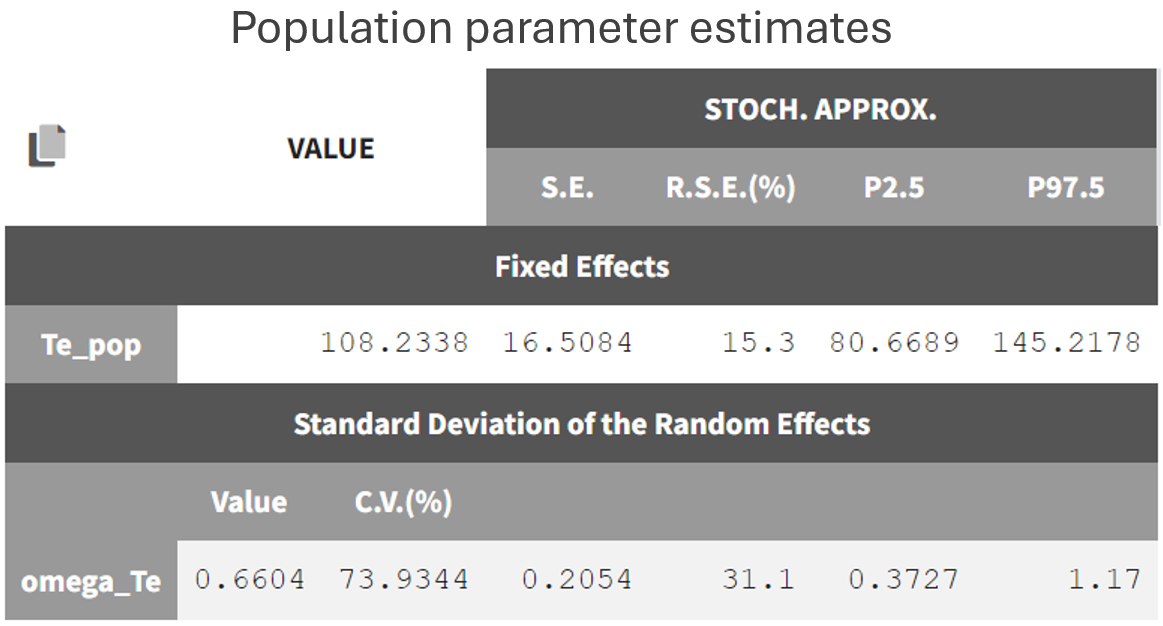
The estimated value, visible in the Results tab, is 109, which is close to the initial estimate.

The standard deviation of the random effects (omega_Te​​) converges to 0.66, corresponding to a coefficient of variation of . The large inter-individual variability likely indicates that sub-populations within the dataset have different Te​ values.

In the next section, covariates will be added to the Te​ parameter to account for this variability and reduce the random effects.

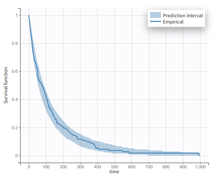
To evaluate whether the exponential model is appropriate, the Visual Predictive Check (VPC) for Time-to-Event data can be reviewed. The figure shows the empirical Kaplan-Meier curve overlaid with the 90% prediction interval based on model simulations. This plot is interpreted similarly to a standard VPC. In this case, the empirical Kaplan-Meier curve falls within the prediction interval, indicating no model mis-specification.

Covariate search

he next step is to determine whether the hazard differs significantly between sub-populations (e.g., those receiving standard treatment versus chemotherapy). Model selection can be approached using various statistical tools, such as information criteria (AIC and BIC) or hypothesis tests (Wald test and likelihood ratio test). In this case study, the Wald test will be used.

Covariates can be incorporated by selecting the appropriate boxes in the “Individual model” section.

The details of the resulting equations can be viewed by clicking on the “f(x)” icon. Adding the categorical covariate "trt" to the parameter Te yields the following:

Adding the continuous covariate "karno" to the parameter TeT_eTe​ results in the following:

Note that this parameterization corresponds to the typical form of a Cox proportional model. Via transformation of the covariates, other forms are also possible.

The parameterization using betas permits to directly perform statistical tests on the beta parameters. In particular, the Wald test tests the following null hypothesis:

The covariate effect on Te​ can be evaluated using different covariate selection methods. One approach is forward selection, where a statistical test, such as the Pearson correlation test or ANOVA, is used to pre-evaluate whether a covariate affects the random effect of the parameter. Alternatively, backward elimination can be applied, where all covariates are included in the model, and the Wald test is used to determine which covariate effects are significantly different from zero and should remain in the model.

Forward selection	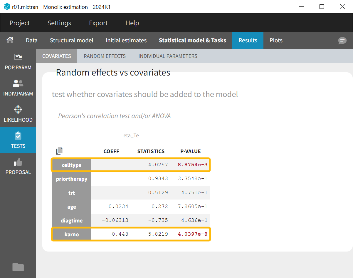Backward elimination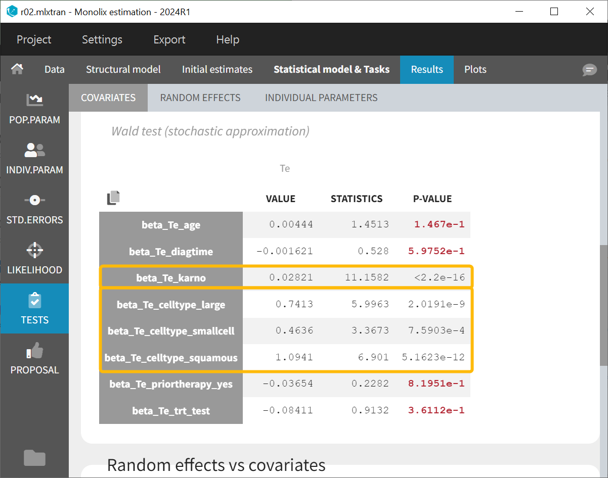

The project run r01.mlxtran on the left side does not include covariates in the individual model, while the project run r02.mlxtran on the right side includes all covariates in the individual model.

Both covariate selection methods lead to the same conclusion: cell type and Karnofsky score have a statistically significant effect on the parameter Te.

In particular, given the data, the new chemotherapy does not significantly lower the risk, compared to the standard treatment.

Next, a model incorporating both Karnofsky score and cell type can be explored.

Since the difference between the “smallcell” and “adeno” cell types (with “adeno” used as the reference in the Wald test) is not significant, as observed in the data plot, these two can be combined into a single category. To add the covariate, use the “Discrete” button to create a new categorical covariate, assigning “adeno” and “smallcell” to the G_adeno_smallcell reference group.

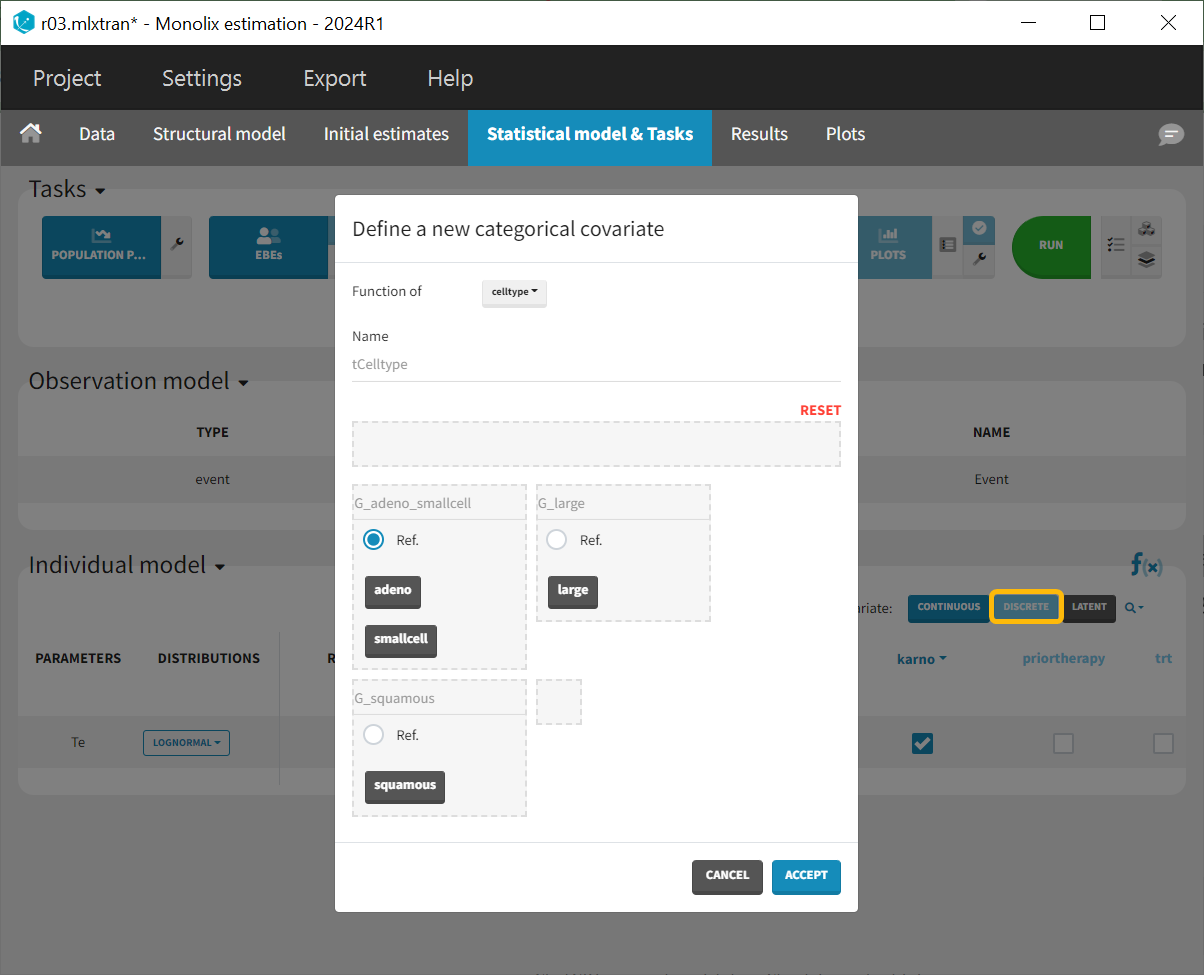
The results are the following:

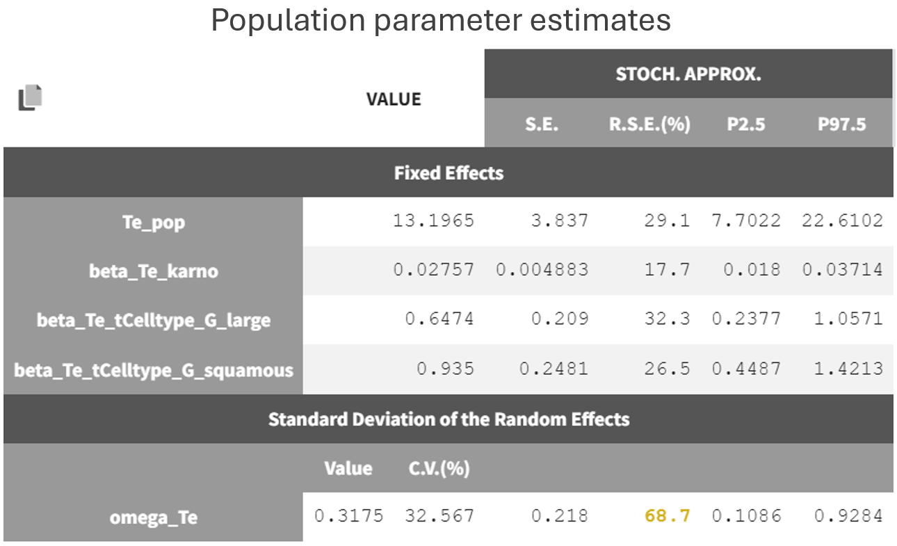
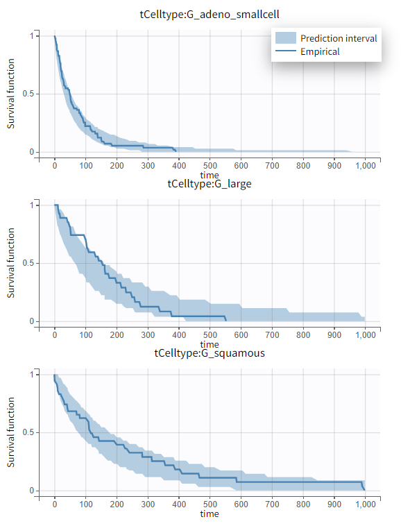
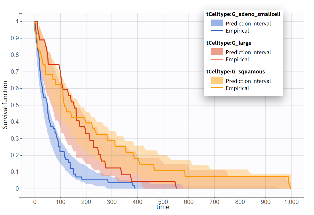
From the estimated beta values, the risk of death is approximately times higher for patients with squamous cell types compared to those with adeno or small cell types. In the graphics, the 95% prediction interval for survival can be stratified by cell type and/or Karnofsky score categories to verify the agreement between the model and the data.

No model mis-specification has been detected; therefore, this model is considered the final model.

The final model is:

For a given cell type and Karnofsky score, the typical hazard and the associated exponential model survival can be calculated analytically:

From the survival function, the probability of surviving at least 1 month (30 days), 3 months (90 days), or 6 months (180 days) can be determined based on the cell type and Karnofsky score.

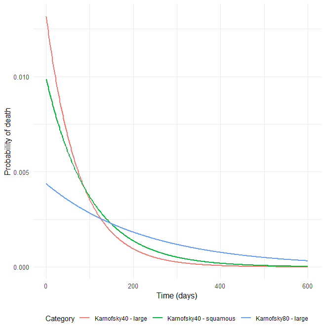
The probability density function of the death event can be calculated for any given Karnofsky score and cell type using , which provides the probability of death over time. For each displayed subpopulation, the plot also shows the distribution of death times within that subpopulation.

Simulations in Simulx

A parametric model for the survival of patients with advanced lung cancer has been developed. This model can now be used to explore the expected survival for new patient cohorts. Simulations are performed using the Simulx application. The Monolix project can be directly exported to Simulx (via Menu/Export/Save and Export to Simulx) and used as input to either simulate the same population as in the original data set or to define new populations.

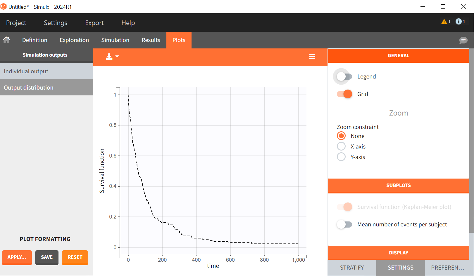
Initially, the same population as in the original data set is simulated. After exporting the Monolix project to Simulx, the simulation scenario in the Simulation tab is configured to re-simulate the original data set.

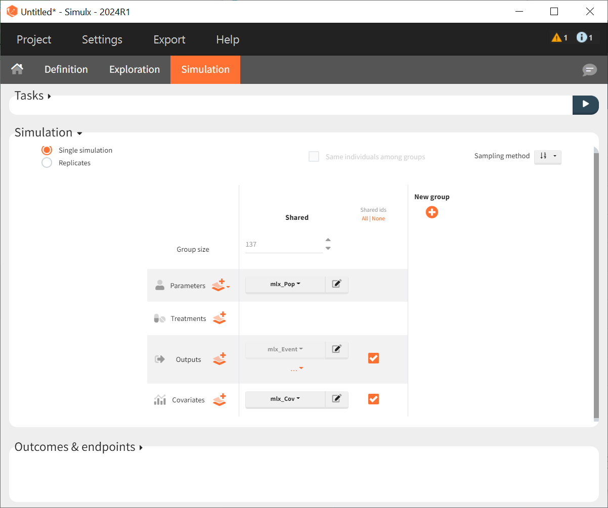
For a given hazard, time of death is a random variable, so the re-simulated Kaplan-Meier survival curve is different compared to the original data.

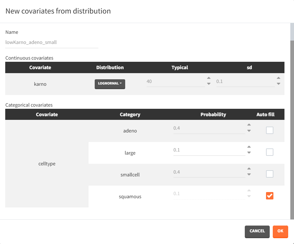
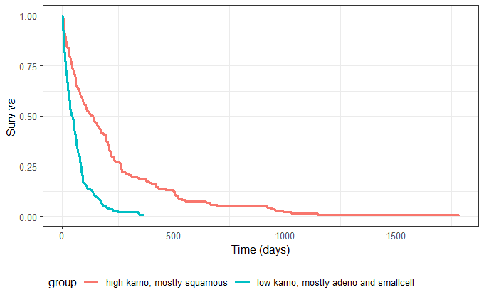
Next, two new patient cohorts are simulated, each with different covariates compared to the original data set. The first cohort consists of patients with a relatively high Karnofsky score, around 70, and a majority of squamous cell types (70% squamous, 10% adeno, 10% smallcell, 10% large). The second cohort includes patients with predominantly adeno or smallcell cell types (40% adeno, 40% smallcell, 10% large, 10% squamous) and a lower Karnofsky score, around 40. The corresponding covariate elements are defined in Simulx with appropriate distributions.

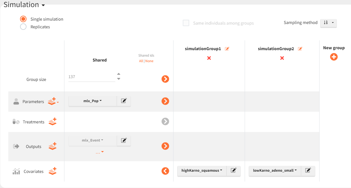
To simulate these two cohorts, two groups are created in the simulation scenario, both using the same population parameters (mlx_pop) and the same observation time (mlx_Event), but with different covariates for the individuals in each group.

The Kaplan-Meier survival curves obtained in these two groups are:

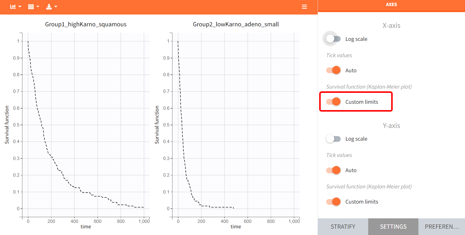
Since the time of death is a random variable, multiple simulations of the same population will produce varying survival curves. The uncertainty of the survival curve can be assessed via replicates, which can be done easily by selecting “Replicates” instead of a “Single simulation” in the simulation tab.

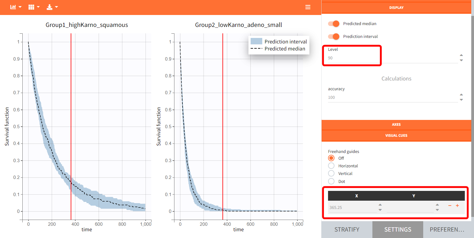
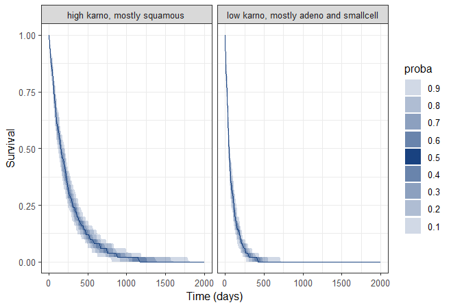
In the figure below, the blue line represents the median Kaplan-Meier curve calculated over 100 replicates, while the shaded area indicates the 90% prediction interval. Visual markers, such as a 1-year survival point, can be added for comparison across different plots.

To quantitatively compare the median survival we use the post-processing tool in Simulx: outcomes & endpoints.

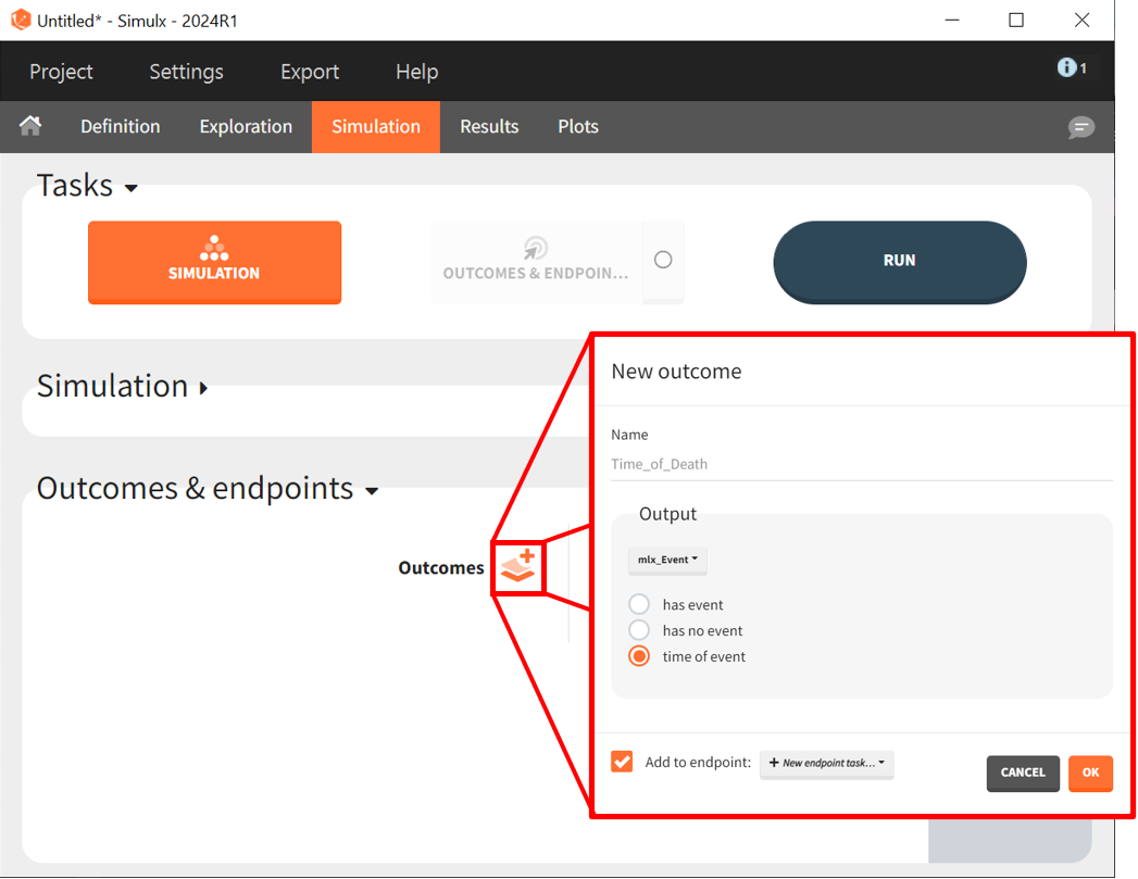
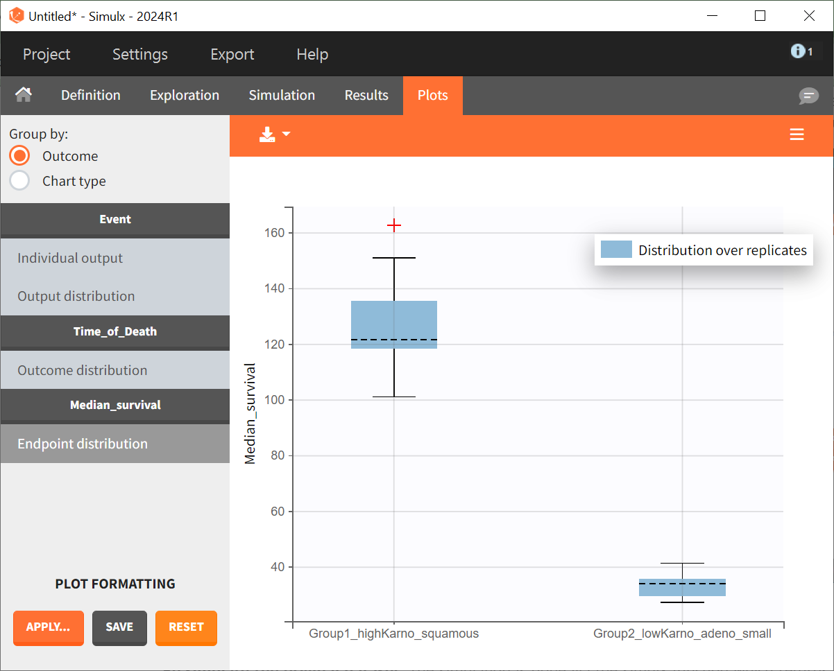
It allows to calculate the median time of event (death) in each group, and asses the uncertainty due to the variability between individuals (when simulating replicates).

The results are presented as a boxplot for the endpoint and in the results tables.

The simulations performed in Simulx can also be conducted in R using either the RsSimulx package or the lixoftConnectors package.

Simulations using lixoftConnectors

All steps needed to set up the new simulation scenario in Simulx, as well as defining outcomes and endpoints, can also be performed in R using relevant functions from the lixoftConnectors package.

This code initializes the MonolixSuite using lixoftConnectors in R, loads a specified Monolix project, and exports it for use in Simulx.

rm(list = ls())
path.prog <- suppressWarnings(dirname(rstudioapi::getSourceEditorContext()$path))
setwd(path.prog)
# GOAL: Simulate treatment scenarios in Simulx to assess outcomes across different populations.

# loading the lixoftConnectors library
library(lixoftConnectors)
path.software <- paste0("C:/Program Files/Lixoft/MonolixSuite2024R1") 

# software initialization: specify the software to be used
initializeLixoftConnectors(path.software,software = "monolix")
options(lixoft_notificationOptions=list(errors=0, warnings=1, info=1))

# loading the final Monolix project
name.project <- "r03.mlxtran" 
path.project <- paste0(file.path(dirname(path.prog),"Monolix"),"/",name.project)
loadProject(projectFile = path.project)

# export monolix project to simulx
exportProject(settings = list(targetSoftware = "simulx", filesNextToProject = T), force=T)

The next step defines two population cohorts: one with a high Karnofsky score (~70) and mostly squamous cell type (70% squamous, 10% adeno, 10% small cell, 10% large), and another with a lower Karnofsky score (~40), predominantly adeno and small cell types (40% each, 10% large, 10% squamous). To incorporate this into the simulation setup, new covariate elements need to be defined. This cannot be done directly with the connector function defineCovariateElement; instead, the required data must first be created in R, then integrated via the connector.

# function to generate Karnofsky score based on typical value and standard deviation
generate_karno <- function(n, typical_value, sigma) {
  karno_values <- rlnorm(n, meanlog = log(typical_value), sdlog = sigma)
  round(karno_values)}

# function to generate celltype values based on specified probabilities
generate_celltype <- function(n, probabilities) {
  sample(names(probabilities), size = n, replace = TRUE, prob = probabilities)}

# set parameters
n <- 137  # number of subjects
sigma_karno <- 0.1  # standard deviation for the lognormal distribution
set.seed(123)  # Set seed for reproducibility

# generate high Karnofsky group data
highKarno_squamous_df <- data.frame(
  id       = 1:n,
  karno    = generate_karno(n, typical_value = 70, sigma = sigma_karno),
  celltype = generate_celltype(n, c(adeno = 0.1, large = 0.1, smallcell = 0.1, squamous = 0.7)))

# generate low Karnofsky group data
lowKarno_adenosmallcell_df <- data.frame(
  id       = 1:n,
  karno    = generate_karno(n, typical_value = 40, sigma = sigma_karno),
  celltype = generate_celltype(n, c(adeno = 0.4, large = 0.1, smallcell = 0.4, squamous = 0.1)))

# save data frames as csv
write.csv(highKarno_squamous_df,      "highKarno_squamous.csv",      row.names = FALSE)
write.csv(lowKarno_adenosmallcell_df, "lowKarno_adenosmallcell.csv", row.names = FALSE)

The csv file containing the new covariate allocations for subjects can be loaded with the defineCovariateElement connector. With a few lines of code, the simulation setup can then be configured, defining outcomes and endpoints similarly to the interface.

# define new covariate element
defineCovariateElement(name ="highKarno_squamous",   element = "highKarno_squamous.csv")
defineCovariateElement(name ="lowKarno_adeno_small", element = "lowKarno_adenosmallcell.csv")

# set simulation scenario
setGroupElement(group = "simulationGroup1", elements = c("mlx_Pop", "mlx_Event", "highKarno_squamous"))
setGroupSize("simulationGroup1",137)
addGroup("simulationGroup2")
setGroupElement(group = "simulationGroup2", elements = c("mlx_Pop", "mlx_Event", "lowKarno_adeno_small"))
setGroupSize("simulationGroup2",137)

# define time to death outcome
defineOutcome(name = "Time_of_Death", element = list(output = "mlx_Event", event = list( type = "timeOfEvents"))) 

# define endpoint 
defineEndpoint(name = "Median_survival",  element = list(outcome = "Time_of_Death",  metric = "kaplanMeier"))

# set simulation and endpoint calculation, define 100 replicates, execute the scenario
setScenario(c(simulation = T, endpoints = T))
setNbReplicates(nb = 100)
runScenario()

To recreate the plots, packages like survival and survminer can be used.

Simulations using RsSimulx function

The documentation on the RsSimulx R-function can be found on this page.

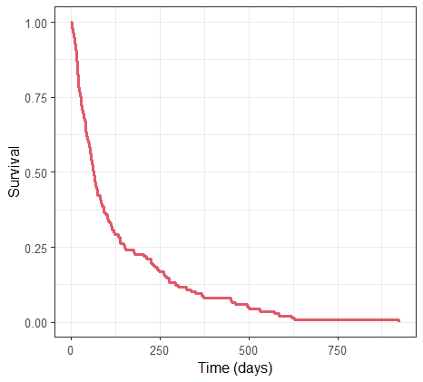
Re-simulate the original data set. The simulation is done via the simulx function which returns an R object containing the result of the simulation (time of death for each individual). The object created is passed into the kmplotmlx function to generate the Kaplan-Meier survival curve:

# loading the RsSimulx library
library(RsSimulx)

# defining the path to the mlxtran project file
project.file <- "./Monolix/r03.mlxtran"

# calling simulx, giving the path to the project as argument
res <- simulx(project = project.file)

# plotting the KM survival curve
kmplotmlx(res$Event) + xlab("Time (days)")

The resulting curve is similar, yet distinct, from the one derived from the original data:

Next, two new patient cohorts are simulated, each with different covariates compared to the original dataset. The first group has a good Karnofsky score (~70) and is mostly squamous cell type, while the second group consists mainly of adeno and small cell types with a lower Karnofsky score (~40). These groups are defined via individual covariate data frames and passed to simulx for simulation. For instance for group 1:

# defining the path to the mlxtran project file
project.file <- "./Monolix/r03.mlxtran"
# defining the a new output element
t <- list(name='Event', time=seq(0, 2000, by=1))
#========== defining group 1
# covariate data frame for group 1, with column id and one column per covariate
cov1 <- data.frame(id=1:137,
                   karno        = rnorm(137,mean=70, sd=5),
                   celltype     = c(rep("squamous",100),rep("large",12),rep("smallcell",12),rep("adeno",13)),
                   diagtime     = rnorm(137,mean=5 ,sd=10),              #unused in model but must be present
                   age          = rnorm(137,mean=62,sd=10),              #unused in model but must be present
                   trt          = c(rep("test",100),rep("standard",37)), #unused in model but must be present
                   priortherapy = c(rep("yes" ,100),rep("no",37)))       #unused in model but must be present 

#============= calling simulx for group 1
res1 <- simulx(project   = project.file,
               covariate = cov1,
               output    = t)

After having put together the results for group 1 and group 2, we obtain the following prediction:

Since the time of death is a random variable, multiple simulations of the same population will produce different survival curves. To assess the uncertainty of the survival curve, replicates can be generated easily by including the argument nrep. This replicates the simulation multiple times, allowing for the assessment of variability across different simulated outcomes.

res1 <- simulx(project = project.file,
               parameter = cov1,
               nrep = 100)

A prediction interval for the two survival curves is obtained:

Conclusion

Monolix allows efficient parametric analysis of this time-to-event (TTE) data set. The risk of death for male patients with advanced inoperable lung cancer is constant over time, fitting an exponential distribution. Prognostic factors include tumor cell type and Karnofsky score. No improvement with the new treatment is evident. The parametric model enables survival probability predictions for specific cell types and Karnofsky scores.

Using Simulx, the developed parametric model can be used for more advanced predictions, to simulate survival for new populations and assess prediction uncertainty through replicates.