Model of double absorption of veralipride

Download data set only | Download all Monolix project files

This case study focuses on modeling the pharmacokinetics of veralipride, a drug known for its double peak plasma concentration after oral absorption.

Site-specific absorption has been proposed as the underlying mechanism for this phenomenon. To explore this hypothesis, a population PK modeling workflow is implemented using the MonolixSuite. The workflow includes direct data exploration and visualization in Monolix to characterize the double peaks, building and estimating two double absorption models within Monolix, assessing the parameter estimates' uncertainty to avoid over-parameterization, and conducting simulations with Simulx to validate the model.

• Introduction and outline

• Data exploration and visualization

• Modeling parallel absorption processes

  • Model selection and initialization for single absorption

  • Model with two first-order absorptions

  • Assessment of parameter estimate uncertainties

  • Adjustment to the residual error model

  • Integrating correlations and assessing estimate robustness

  • Predictive power of the final model

• Double absorption site model

  • Model writing with macros and ODEs

  • Model exploration with Simulx

  • Model estimation and diagnosis with Monolix

• Simulations and model validation

  • Simulations with Simulx

  • Simulations and post processing with lixoftConnectors

• Conclusion

Note, the video was recorded with MonolixSuite version 2018. Many updates have been made since, but the overall workflow remains the same across versions.

Introduction

Veralipride is a benzamide neuroleptic medicine indicated in the treatment of vasomotor symptoms associated with the menopause. This case study is based on a data set of veralipride PK measured on 12 individuals, published in:

Plusquellec, Y, Campistron, G, Staveris, S, Barre, J, Jung, L, Tillement, JP, Houin, G (1987). A double-peak phenomenon in the pharmacokinetics of veralipride after oral administration: a double-site model for drug absorption. J Pharmacokinet Biopharm, 15, 3:225-39.

Multiple peaks in plasma concentration-time curves is not uncommon, but it can create difficulties in the determination of PK parameters. This phenomenon can be explained by different physiological processes. Some are discussed for example in the review:

Davies, NM, Takemoto, JK, Brocks, DR, Yáñez, JA (2010). Multiple peaking phenomena in pharmacokinetic disposition. Clin Pharmacokinet, 49, 6:351-77.

• solubility-limited absorption, due to pH-specific differences between segments along the length of the gastrointestinal tract,

• complexation with poorly absorbable bile salt micelles in the proximal part of the small intestine,

• sustained-release formulations designed to have both a fast- and a slow-release component,­­

• enterohepatic recycling: biliary secretion followed by intestinal reabsorption of a drug,

• delayed gastric emptying,

• variability of absorption of drugs through the gastrointestinal membrane, due to biochemical differences in the regional areas of the gastrointestinal tract,

• effects of surgery and anaesthesia: it has been postulated that enhanced muscle blood flow occurring upon recovery from anaesthesia could contribute to increased plasma concentrations.

In the case of veralipride, site-specific absorption has been suggested to be the major mechanism responsible for the multiple peaking phenomenon, with rapid absorption occurring in the proximal part of the gastrointestinal tract, followed by a second absorption phase in more distal regions. This hypothesis was tested with the use of a telemetric shuttle for site-specific administration of the drug into the small intestine.

Different modelling attempts for veralipride have been published. They follow two main modelling approaches:

• The first approach uses double absorption models, assuming simultaneous input via two parallel pathways. This lacks a biological justification linked to physiology.

• The second approach strives to ensure a clear physiological interpretation. Thus, this approach uses models with two successive absorption windows. In order to define each time phase, the model used in this case study requires one more parameter than for the first approach.

In this case study we will explore both approaches with MonolixSuite.

Case study outline

The data set is explored within Monolix. This graphical exploration characterizes several properties of the dataset, including the presence of double peaks in plasma concentrations for some individuals and the elimination phase.

In section “Modeling parallel absorption processes“ a model featuring parallel first-order absorption is applied, adapted from a single absorption model available in the PK library. A step-by-step approach is taken to estimate parameters, diagnose the model, and implement necessary adjustments. Given the limited number of individuals in the data, alongside the model's requirement for numerous parameters, it is crucial to assess the uncertainty of parameter estimates to avoid over-parameterization. Specific attention is given to adapting the settings of SAEM to accurately identify inter-individual variability, as well as utilizing the correlation matrix of estimates and convergence assessments to recognize potential over-parameterization.

In section “Double absorption site model“ A model from the literature (Godfrey et al.,  2011) is evaluated, which assumes a discontinuous input rate of the drug at two absorption sites. Instructions are provided on how to implement this model in Monolix using ODEs or PK macros. The model's behavior is subsequently explored with Mlxplore. Finally, a modeling workflow is established in Monolix to estimate and diagnose the model.

The first model is selected to perform new simulations in Simulx, aiming to assess the drug's effects in various ways within a large population.Data exploration and visualization

Data exploration and visualization

The data set has been originally published in:

Plusquellec, Y, Campistron, G, Staveris, S, Barre, J, Jung, L, Tillement, JP, Houin, G (1987). A double-peak phenomenon in the pharmacokinetics of veralipride after oral administration: a double-site model for drug absorption. J Pharmacokinet Biopharm, 15, 3:225-39.

100 mg doses of veralipride were given to 12 healthy volunteers by oral solution. Individual plasma concentrations of veralipride (ng/ml) were observed during 24h (time is measured in h) after the administration. Doses were given in the morning after an overnight fast, and subjects fasted up to 4 hr after drug administration in each case.

The columns are:

• ID: the subject ID, column-type ID.

• TIME: the time of the measurement or of the dose, column-type TIME.

• AMT: the amount of drug provided to this subject, column-type AMOUNT

• Y: the measurement, column-type OBSERVATION.

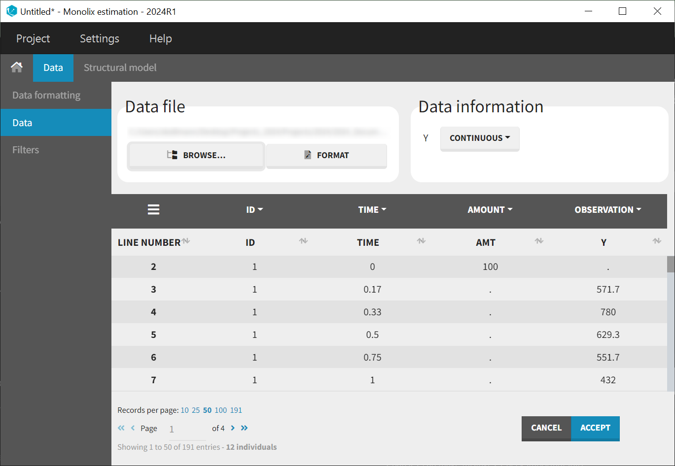
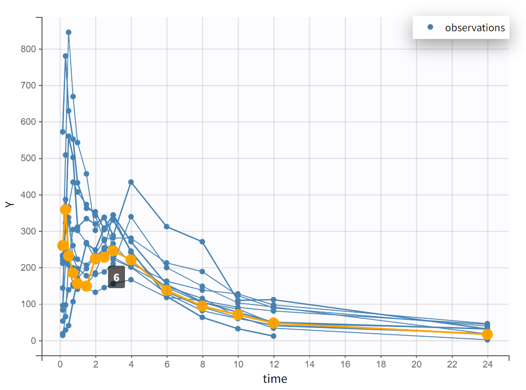
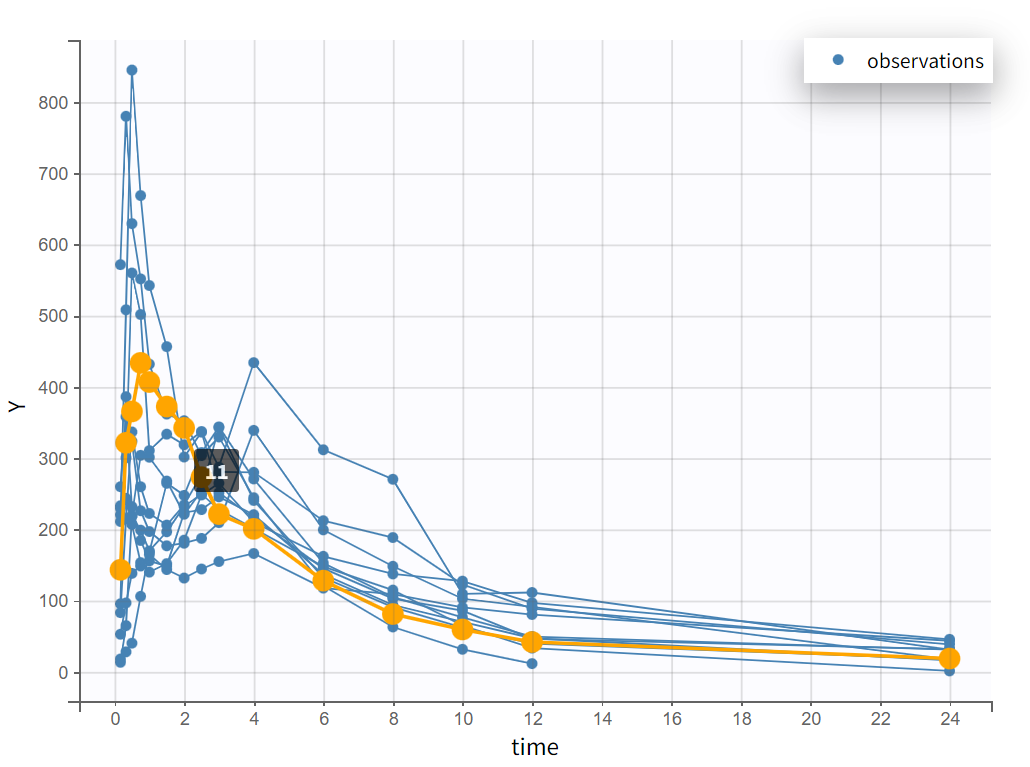
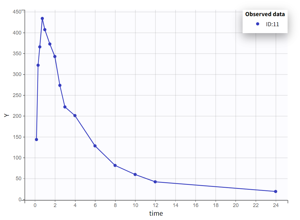
After creating a new project, the dataset is loaded with the default column types. A plot of observations versus time is generated and displayed in the figure below, highlighting an example of an individual exhibiting a double peak in plasma concentrations.

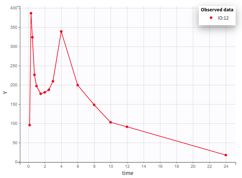
Focusing on each individual with the individual selection in the Stratify panel allows to check that the second peak is not always measured as smaller than the first peak.

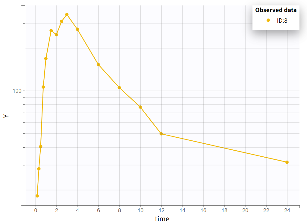
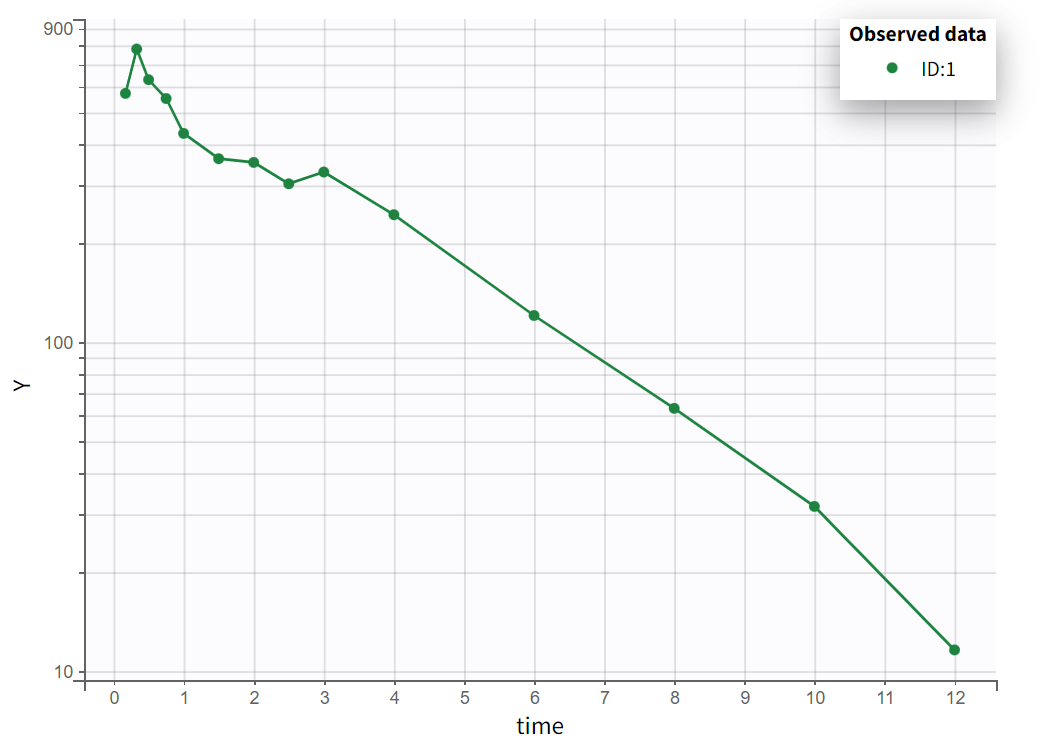
Choosing a log-scale on the Y axis is useful to focus on the elimination phase for each individual. Some of the individual curves seem to display an elimination phase with two slopes, characteristics of a two-compartments model. This is for example the case for the individual 8 as seen below (left), but not for individual 1 (below, right) which seems close to a linear elimination.

In conclusion, this graphical exploration identified several properties:

• Nine out of twelve individuals exhibit a double peak in plasma concentrations.

• The second peak is not consistently smaller than the first.

• Some individual curves appear to display an elimination phase with two slopes, characteristic of a two-compartment model.

Modeling parallel absorption processes

Model selection and initialization for single absorption

To help initializing the parameter estimates, a model with one absorption will be estimated before adding the second one. Data exploration indicated that a two-compartment model may be necessary for some individuals. Therefore, the starting point is a model featuring two compartments, first-order absorption, and linear elimination. This model is available in the PK library with different parameterizations. The model encoded with rates, oral1_2cpt_kaVkk12k21.txt, is selected.

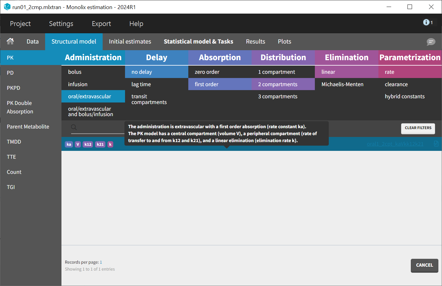
After choosing the model, the tab “Initial estimates” allows to choose initial values for the five population parameters. The initialization has been performed using the auto-init function, which automatically identifies a good fit to establish suitable starting points. The log scale selected for the Y axis permits to check that two slopes are visible for the elimination, characterizing the second compartment.

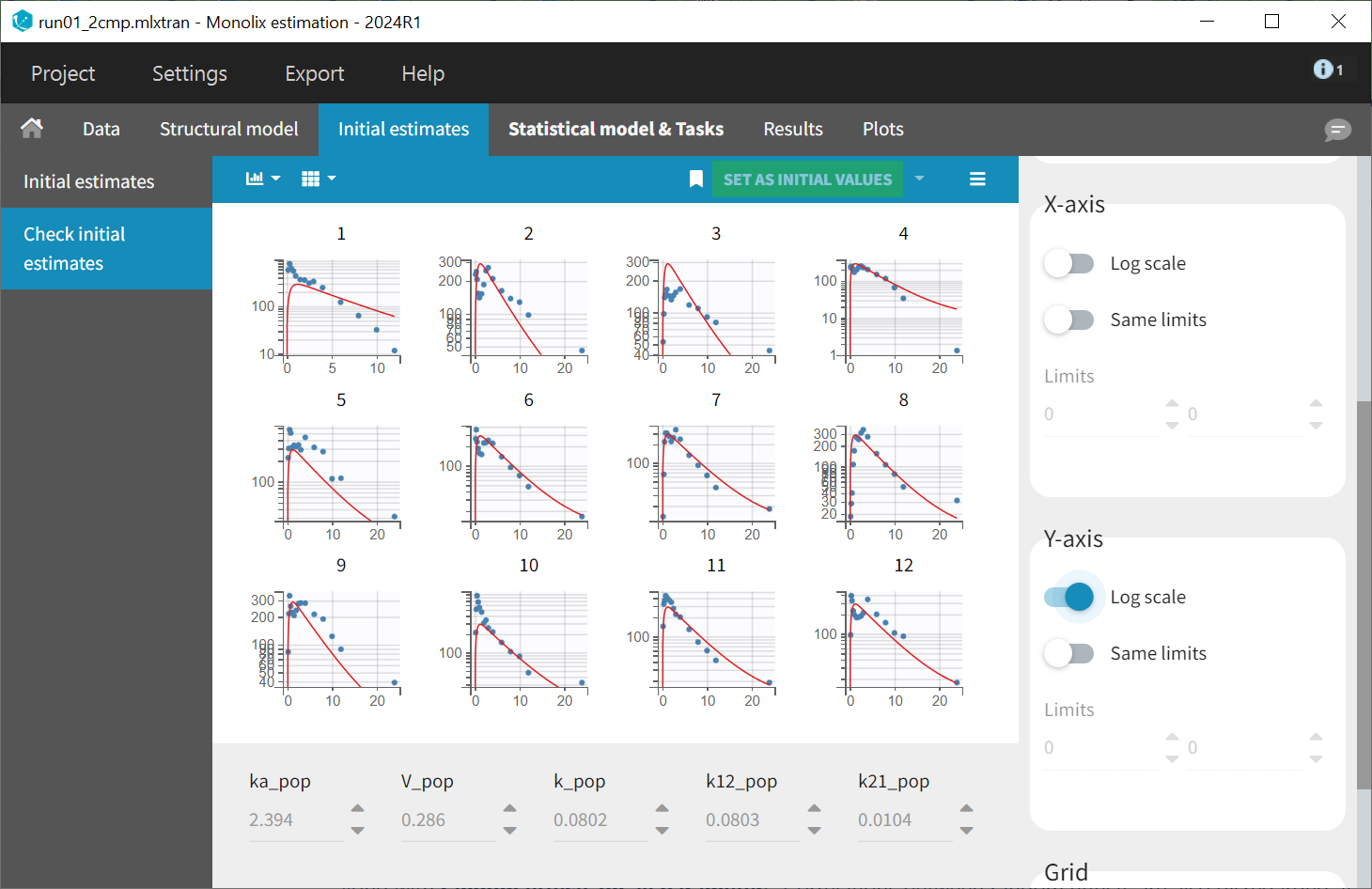
Initial values are validated by selecting the green "Set as initial values" button. The "Statistical model & Tasks" tab then appears, which can be used to adjust the statistical model and run tasks to evaluate the full model.

In this initial modeling phase, the goal is to build the structural model in several steps, so the default statistical model is retained for now. This model comprises a combined residual error model with both additive and proportional terms, log-normal distributions for the five parameters and along with random effects on all parameters. Correlations between random effects are also disregarded at this stage.

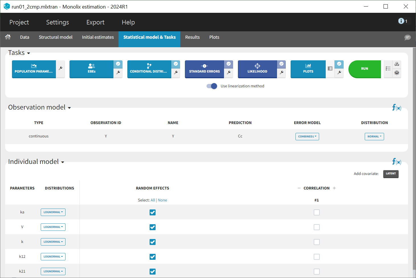
Once all the elements of the model have been specified, several tasks can be run in the “Statistical model & Tasks” tab to estimate the parameters and evaluate the fit to the data. It is important to save the project before (Menu > Save > run01_2cmp.mlxtran), so that the result text files of all tasks run afterwards will be saved in a folder next to the project file.

To quickly evaluate the model, the tasks “Population parameters” and “EBEs” are selected in the scenario to estimate both population parameters and individual parameters. The task “Conditional Distribution” is also chosen, as it enhances the performance of the diagnostic plots, particularly when dealing with a small number of individuals, as is the case here. Additionally, the task “Plots” is selected to facilitate model diagnostics. The scenario can then be executed by clicking on the green 'Run' button.

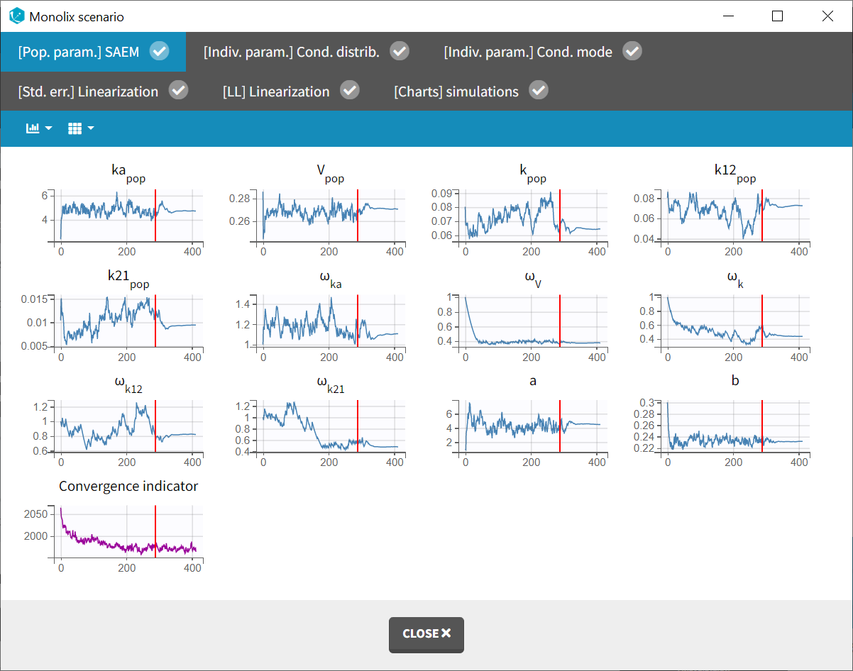
The “Monolix scenario” window provides real-time monitoring of the progress for each task. In particular, the graphical report of SAEM iterations is useful for evaluating convergence.

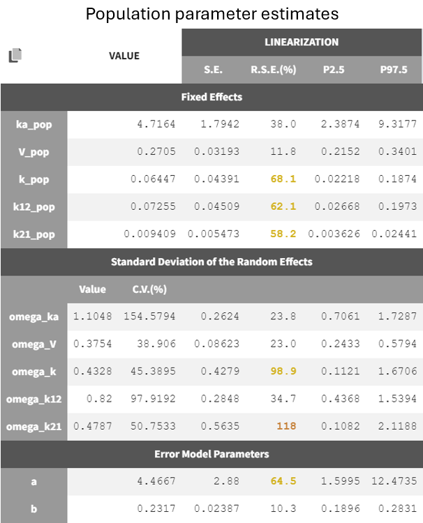
Two new tabs now display the results of the tasks. The tab “Results” contains the estimated parameters as tables, for example the population parameters shown below. Some fixed effect parameters, like and , have borderline elevated RSEs. These parameters are relate to distribution and elimination in the concentration-time profile, which may be due to the fact that only a few subjects show a second slope in the log-scaled elimination phase. Additionally, the associated omega parameters, and , also have high RSEs

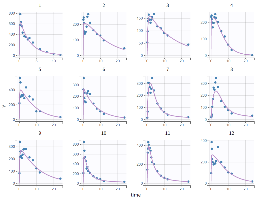
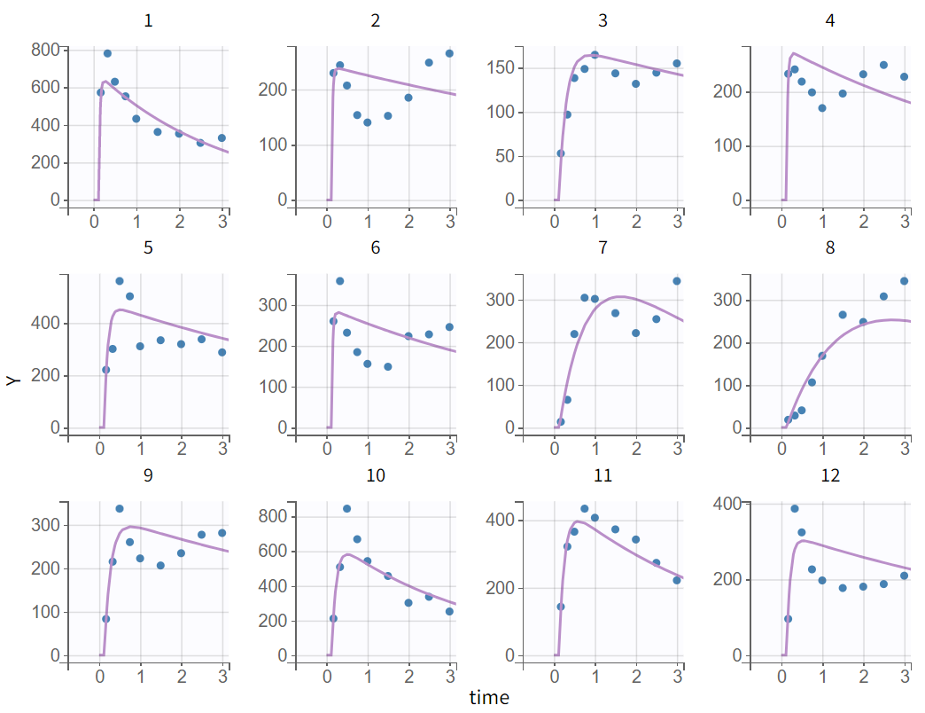
The tab “Plots” contains the diagnostic plots. Among these, the plot “Individual fits”, displayed on the figure below, allows to see that rough individual fits have been found with this first model, that do not capture the double peaks but fit properly the elimination.

It is visible that the prediction curve does not match the higher concentrations, as the observed data points at these levels are consistently under-predicted.

On the "Observations vs. Predictions" plot shown below in log-log scale, several over-predicted outliers are visible outside the 90% prediction interval. This suggests potential mis-specification of the structural model. The interactive plot allows identification of the corresponding individuals: hovering over a dot reveals the ID and time, and highlights all the dots for that individual.

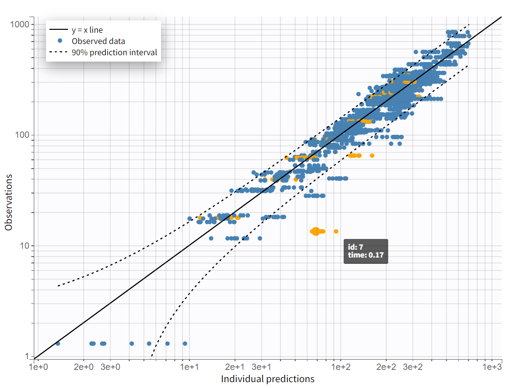
Notice that each time point corresponds to several dots, corresponding to different predictions for one observation, based on different individual parameters drawn from the conditional distribution. This method circumvents the phenomenon of shrinkage.

Most outliers correspond to early time points: 0.17h for the individuals 7, 10 and 12, 0.33h for the individual 7 and 8, and 0.5h for individual 8.

Returning to the individual fits plot, the linked X-axis zoom allows focusing on early time points for all individuals. The X-axis interval can also be adjusted in the "Axes" section of the "Settings" panel.

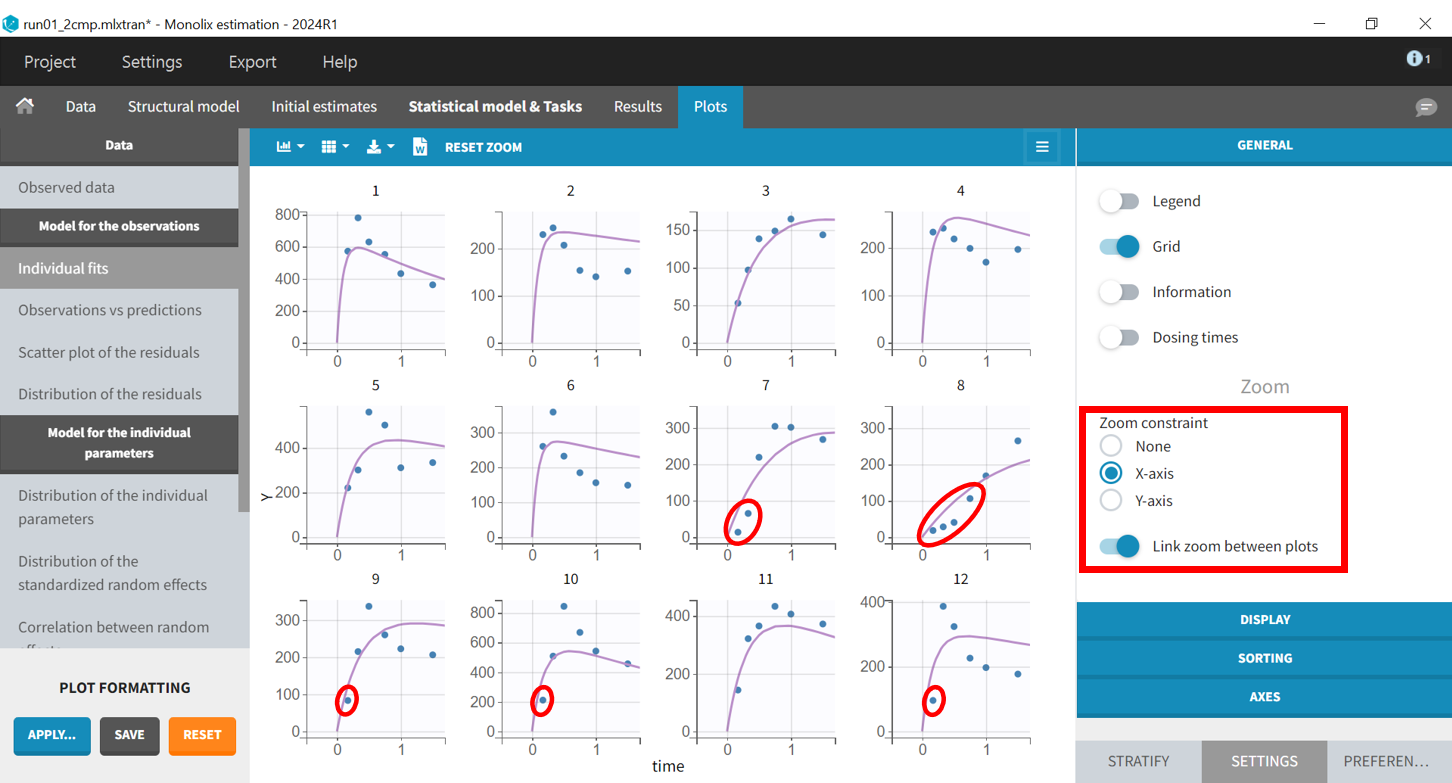
The predicted absorption begins too early for individuals 7, 8, 9, 10, and 12, leading to over-predictions at low times. This indicates the need to include a delay for oral absorption in the structural model.

Before modifying the structural model, it is possible to use the population estimates as new initial values to accelerate convergence. This can be done by clicking "Use last estimates: Fixed effects" in the "Initial estimates" tab. Then, in the "Structural model" tab, a new model from the library is selected with delayed first-order absorption: oral1_2cpt_TlagkaVkk12k21.txt.

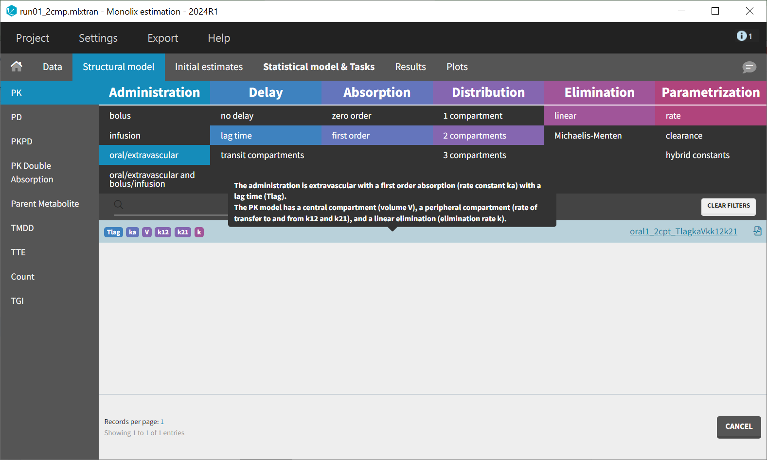
This model introduces an additional parameter, Tlag, compared to the previous one. In the "Initial estimates" tab, a reasonable initial value for can be set. Based on the individual fits, this value should be between 0 and 0.17, with 0.1 being a suitable choice. The initial values for the other five parameters remain unchanged from the previous estimates.

The modified project can be saved as run02_2cmp_Tlag.mlxtran, and the same scenario can be executed.

As shown in the results, the estimates for and remain close to the previous values, while has increased. The RSEs for and have decreased, while for and , they have increased.

Zooming in again on the early time points of the absorption phase in the “Individual fits“ plot, the earliest observations are now better captured by the prediction curve.

The plot “Observations vs predictions”, pictured below, now shows much less outliers.

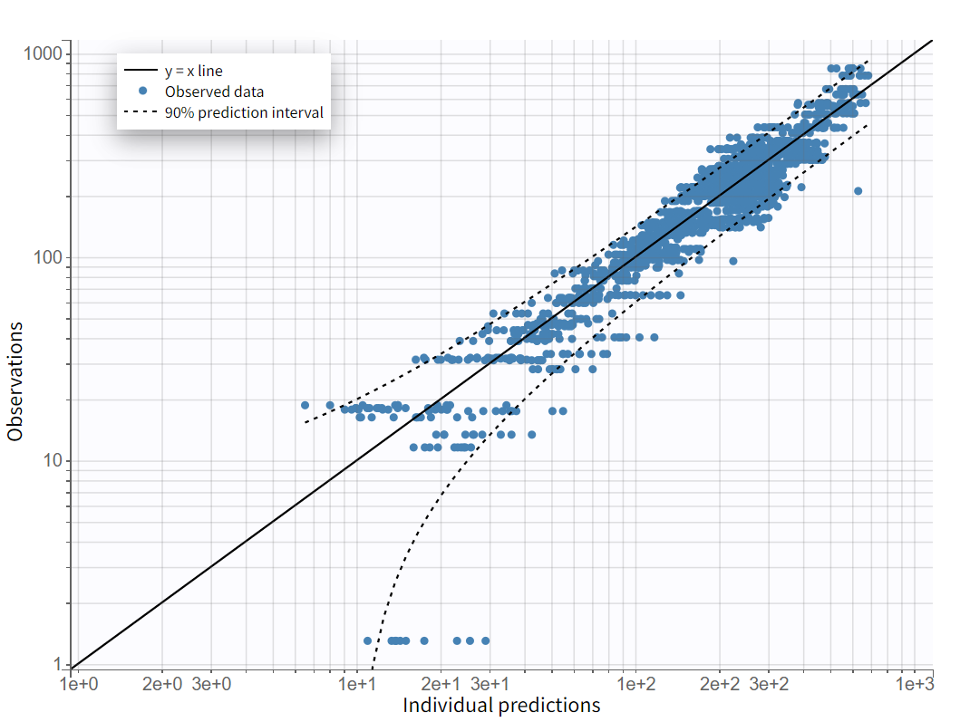
No significant mis-specifications are visible, aside from the second absorption peak observed in some individual curves, as previously noted in the “Observed data“ plot. To capture this, a second delayed first-order absorption can be included in the structural model.

Model with two first-order absorptions

As before, the population estimates are kept as new initial values by selecting "Use last estimates" in the "Initial estimates" tab. The structural model is then modified. A model from the library of “PK Double Absorption” in Monolix (available since version 2019) is selected.

The following filters are applied: delay = "lag time" and type = "first order" for both absorption phases, with "force longer delay" set to "true" for the second absorption, distribution = "2 compartments," and elimination = "linear".

The model is written using PK macros and reads as follows:

[LONGITUDINAL]
input = {ka1, ka2, F1, Tlag1, diffTlag2, V, k, k12, k21}

EQUATION:
odeType=stiff

; Parameter transformations
Tlag2 = Tlag1 + diffTlag2

PK:

;PK model definition
compartment(cmt = 1, volume = V, concentration = Cc)
absorption(cmt = 1, ka = ka1, Tlag = Tlag1, p = F1)
absorption(cmt = 1, ka = ka2, Tlag = Tlag2, p = 1-F1)
peripheral(k12, k21)
elimination(cmt = 1, k)

OUTPUT:
output = Cc
table = Tlag2

Each dose is divided into two fractions, and , which are absorbed through first-order processes with distinct absorption rates and delays. The parameter transformation for Tlag2 guarantees that the second absorption begins after the first. In Monolix, only is estimated; however, the value for will be accessible in the results folder through the table statement.

The implementation with PK macros takes advantage of the analytical solution if it is available, which is the case here. Note that the syntax for each section of a Mlxtran model, such  INPUT, OUTPUT or PK, is documented here.

After loading the model, initial values have to be chosen for the new parameters. Here, ka and Tlag have also been renamed into ka1 and Tlag1, so ka1_pop and Tlag1_pop are considered as new population parameters.

For double absorption models, setting initial values can be challenging. Reviewing the observed data in the individual fits reveals that seven individuals (Subjects 1, 5, 6, 9, 10, 11, 12) show a higher first peak, three individuals (Subjects 2, 7, 8) have a higher second peak, and two individuals exhibit approximately equal peaks. Since about 60% of the population has a higher first peak, a lower initial value is assigned for ka2 compared to ka1 in the parameter initialization. Therefore, is set to 12 and to 4

=0.12, which is approximate to previous estimates for. can also be inferred from the observed data in the individual fits plot. Zooming in on the early phase of the absorption process in the time profile shows that the rise towards the second peak starts around 2 hours. is not a parameter measured directly but is reflected by the parameter . Therefore, is set to approximately 1.88, so that with , equals 2. For =0.8 is selected. These values just serve as a starting point for the algorithm, the final estimated value may differ after the estimation process.

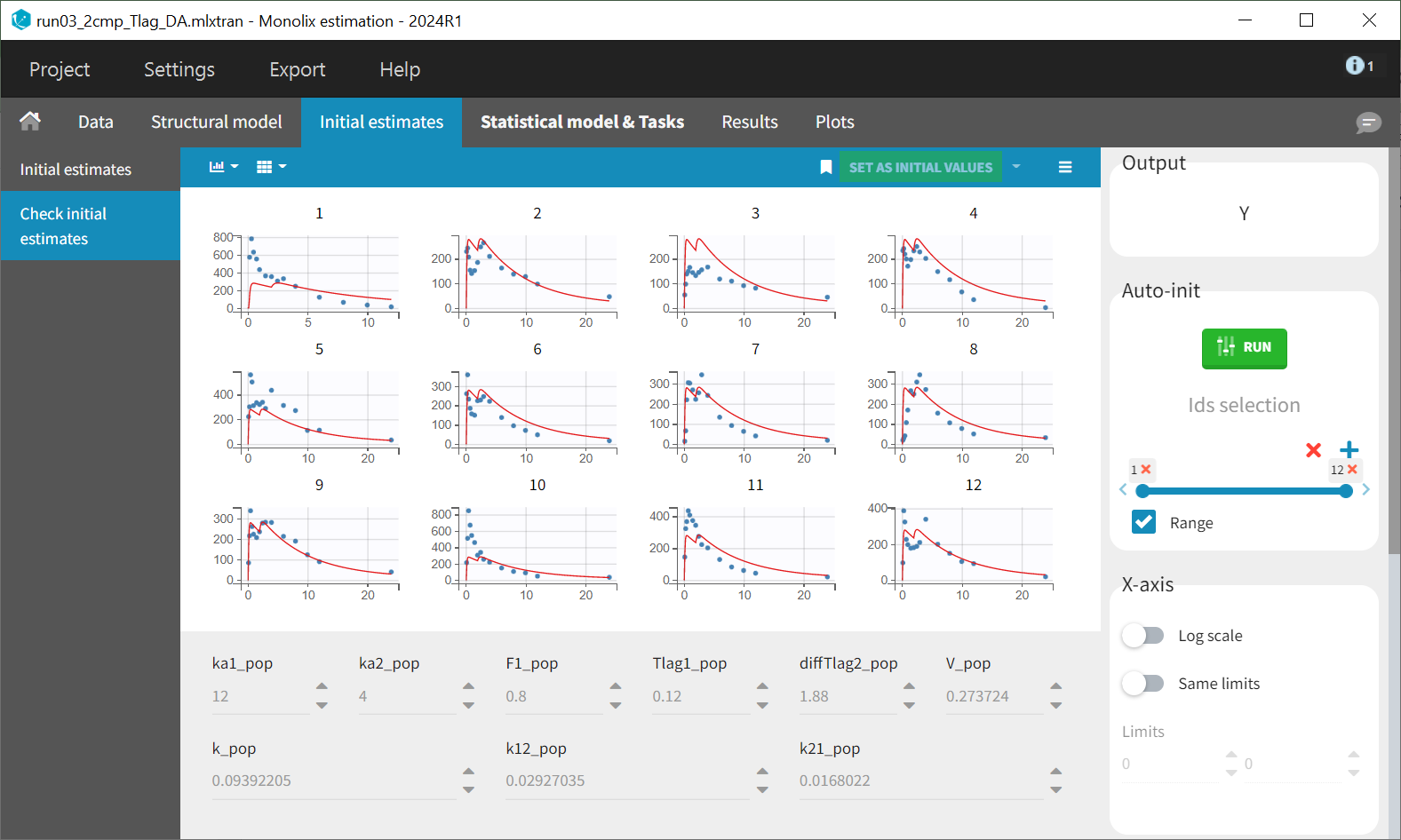
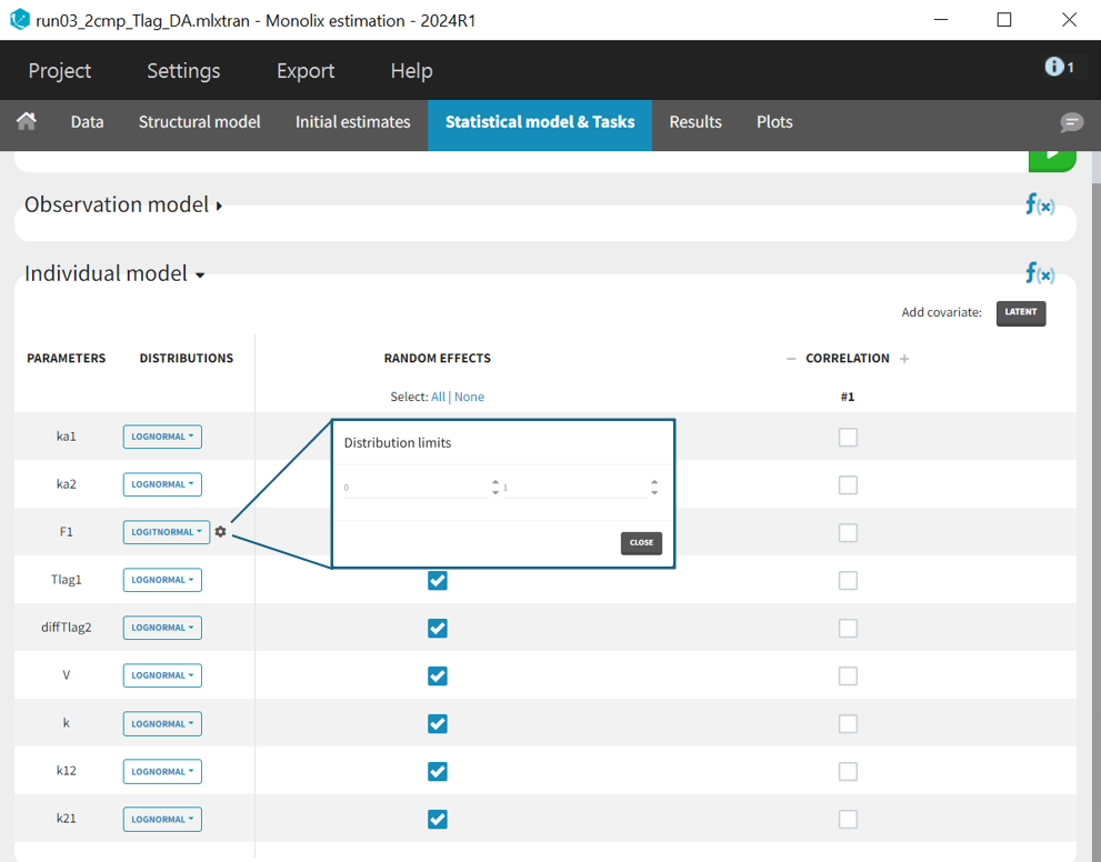
The individual parameter F1 represents a fraction and must remain between 0 and 1. To ensure this, its distribution is automatically set to a logit-normal distribution in the individual model (see screenshot below), as it is a model from the library. The updated project is then saved as run03_2cmp_Tlag_DA.mlxtran.

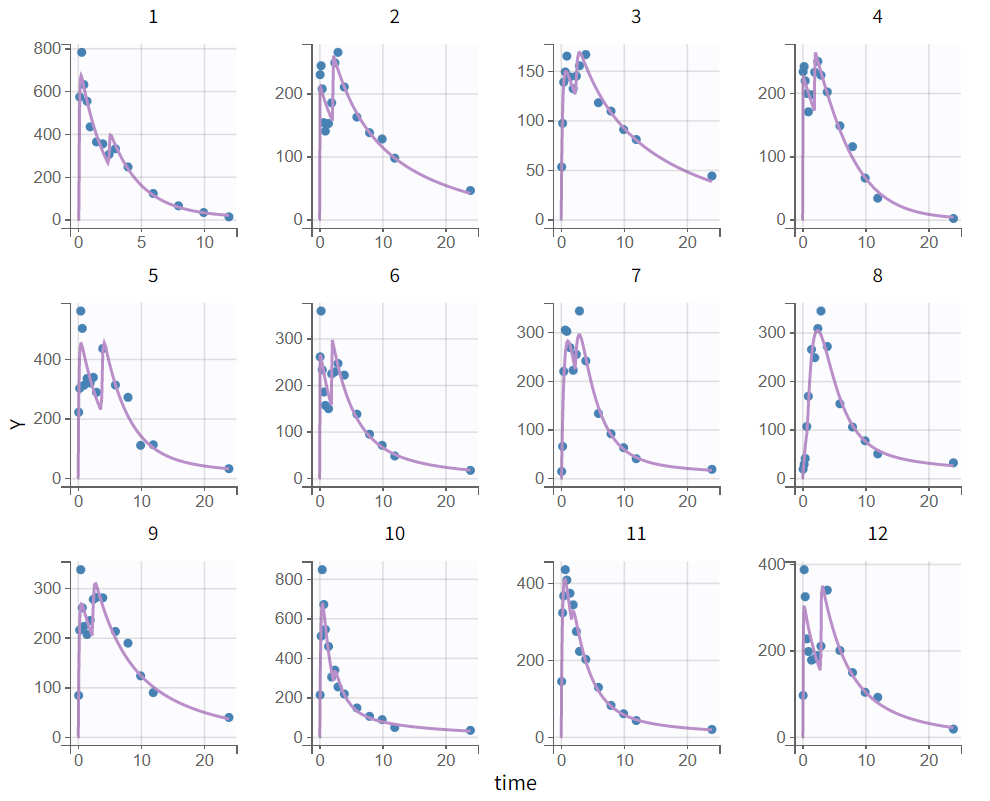
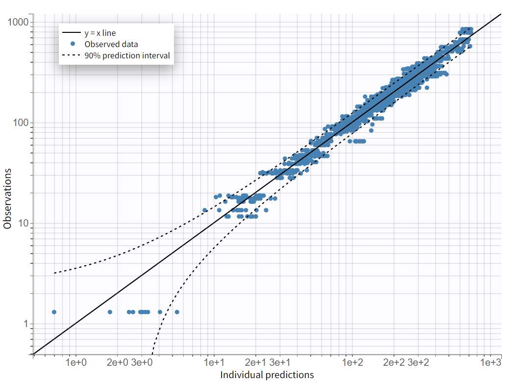
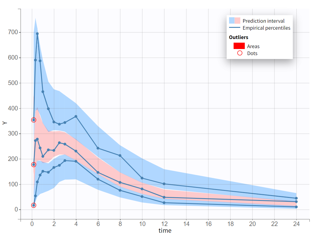
After rerunning the same scenario, the estimates of the distribution and elimination parameters are very similar to the parameter estimates from the previous run. Moreover, they have been estimated with good certainty. The new parameters are also approximately in the range in which they were initialized, again with relatively good certainty. Regarding model diagnostics, although the high concentrations in the individual fits were not captured by the prediction curve in most profiles, the observations versus predictions plot and the VPC do not indicate any visible misspecifications.

Assessment of parameter estimate uncertainties

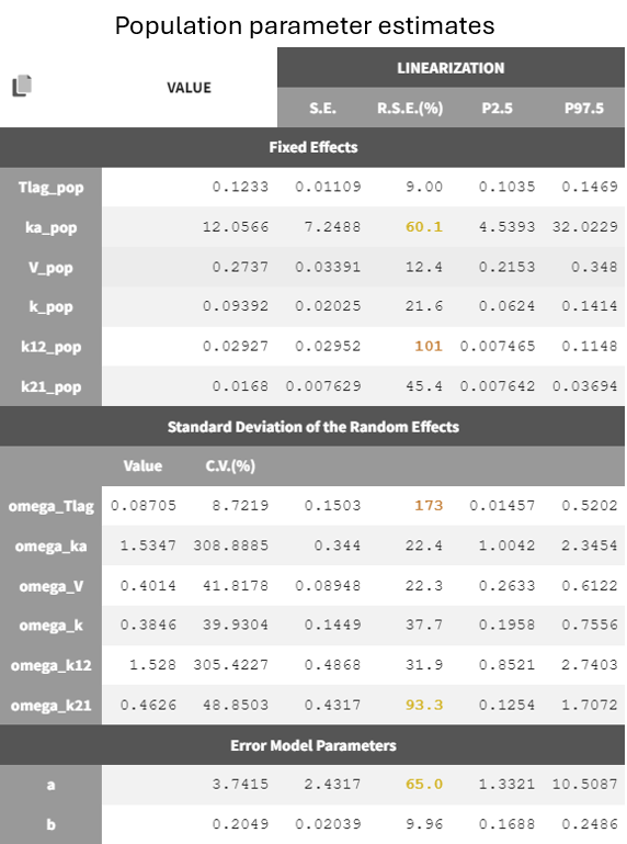
The uncertainties of the population estimates are assessed by executing the "Standard errors" task. For a rapid assessment, the linearization method is selected, which quickly computes the standard errors, shown in the table of population parameter estimates.

The uncertainty of the parameter estimates aids in evaluating the model. The final structural model run shows borderline high relative standard errors for the fixed effects and . The same applies to the omega parameters and , as well as the constant error model parameter , which has one of the highest R.S.E.s.

This model seems to describe the key features of the profiles well, with relatively reasonable estimates, but a convergence assessment can check the stability of the parameter estimates and thus the predictions.

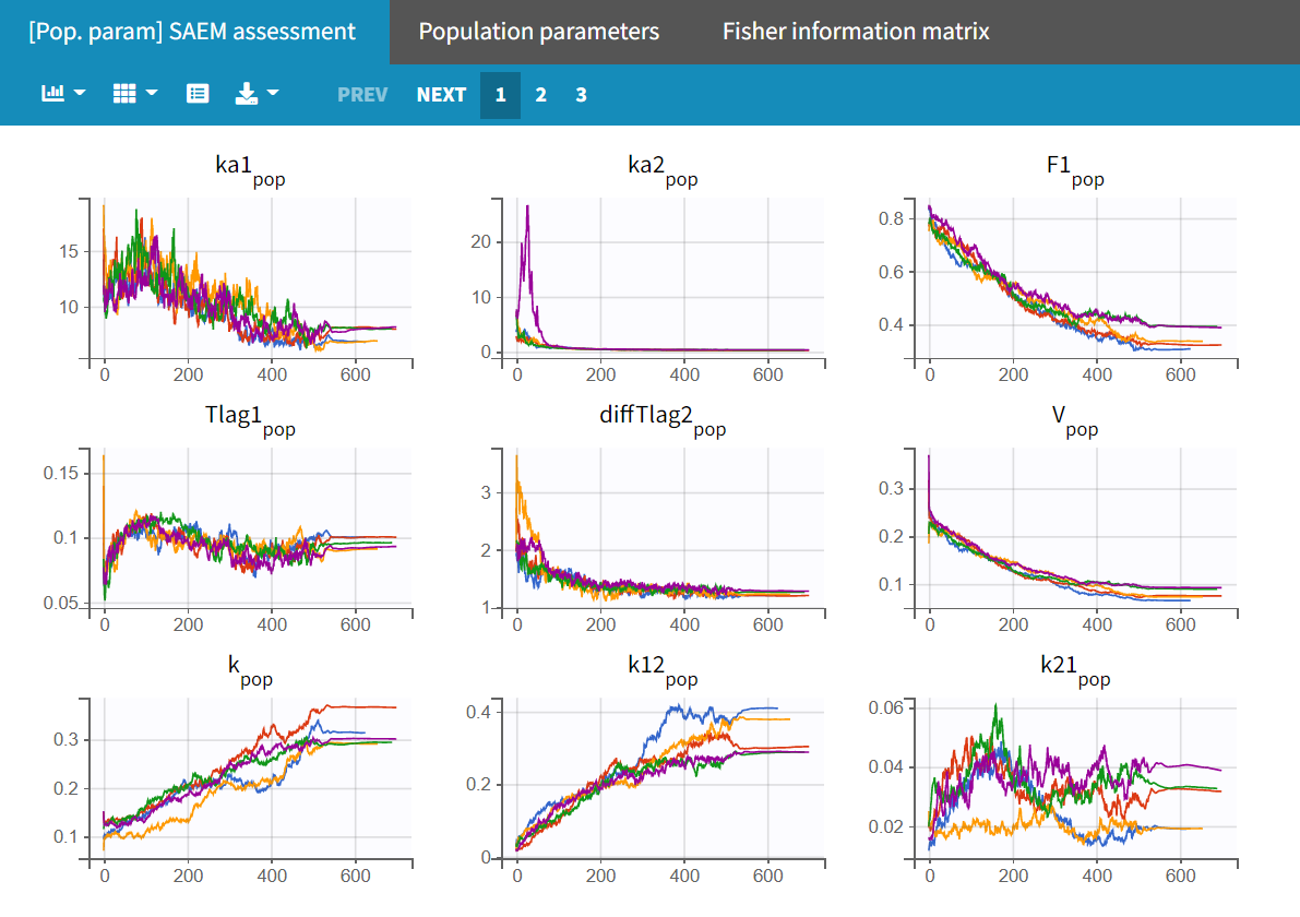
The convergence assessment allows you to set the number of runs, estimate the standard error and log-likelihood and also whether sensitivity to the initial values should be taken into account. This means that initial values are drawn evenly from intervals around the estimated values for all fixed effect parameters, so that each run has different initial values.

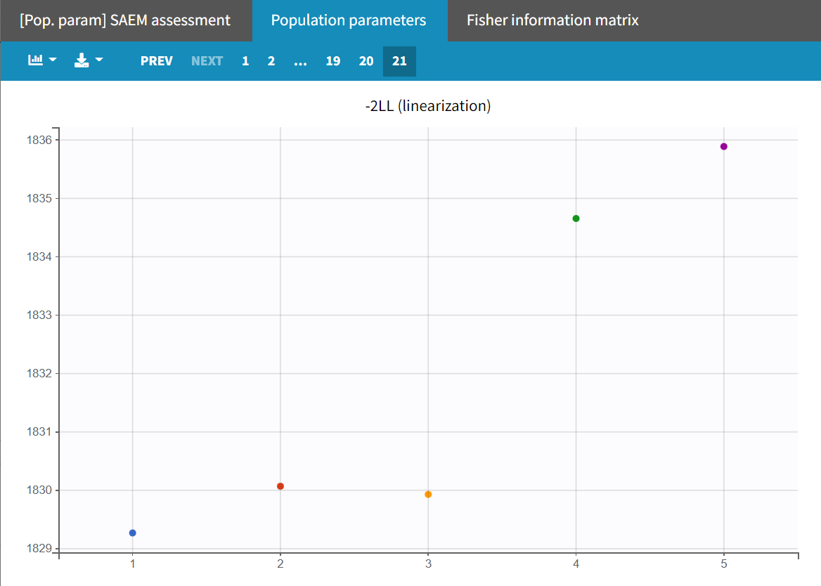
In the "Run" tab, the trajectory plots for the different runs can be viewed under "[Pop.param] SAEM assessment." The "Population parameters" plot displays the final parameter estimates for each run along with their corresponding standard errors.

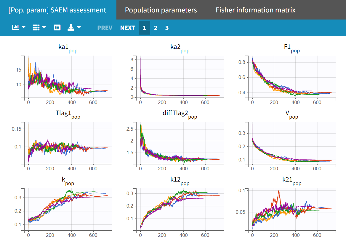
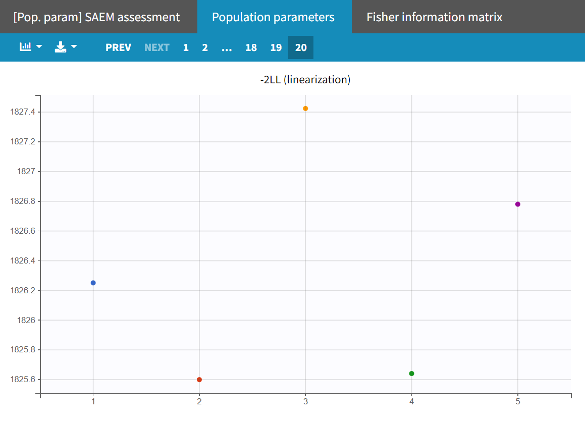
Upon closer examination, the trajectories of the fixed effects show that the algorithm converges to different values across different runs. Additionally, the estimated log-likelihoods vary, with a maximum difference of about 6 points between runs. This indicates that the estimates are not very stable, and the model requires further refinement.

High R.S.E.s in parameter estimation, along with an unstable -2LL estimate in the convergence assessment, indicate that the estimates are too uncertain. Removing variability may have a beneficial effect on the predictions. To determine which random effects should be removed, the standard deviations of the random effects will be estimated more precisely by running the population parameter estimation with SAEM without simulated annealing. This method may also help identify other random effects that can be removed from the model.

This approach is explained in detail in this video, but here is a brief summary:

By default, SAEM includes a simulated annealing method, which gradually reduces the variance of the random effects and residual error parameters. The maximum reduction between iterations is 5% by default. This method is useful in the early stages of the modeling workflow because the size of the parameter space explored by Monolix depends on the omega values. Keeping these values high allows the SAEM algorithm to explore a larger parameter space and avoid getting stuck in local minima, promoting convergence toward the value of maximum likelihood.

However, after finding good initial values and minimizing the risk of local minima, simulated annealing may keep omega values artificially high, even after many SAEM iterations, preventing the identification of parameters with zero variability. At this point in the workflow, disabling simulated annealing in the 'Population parameters' task settings can help.

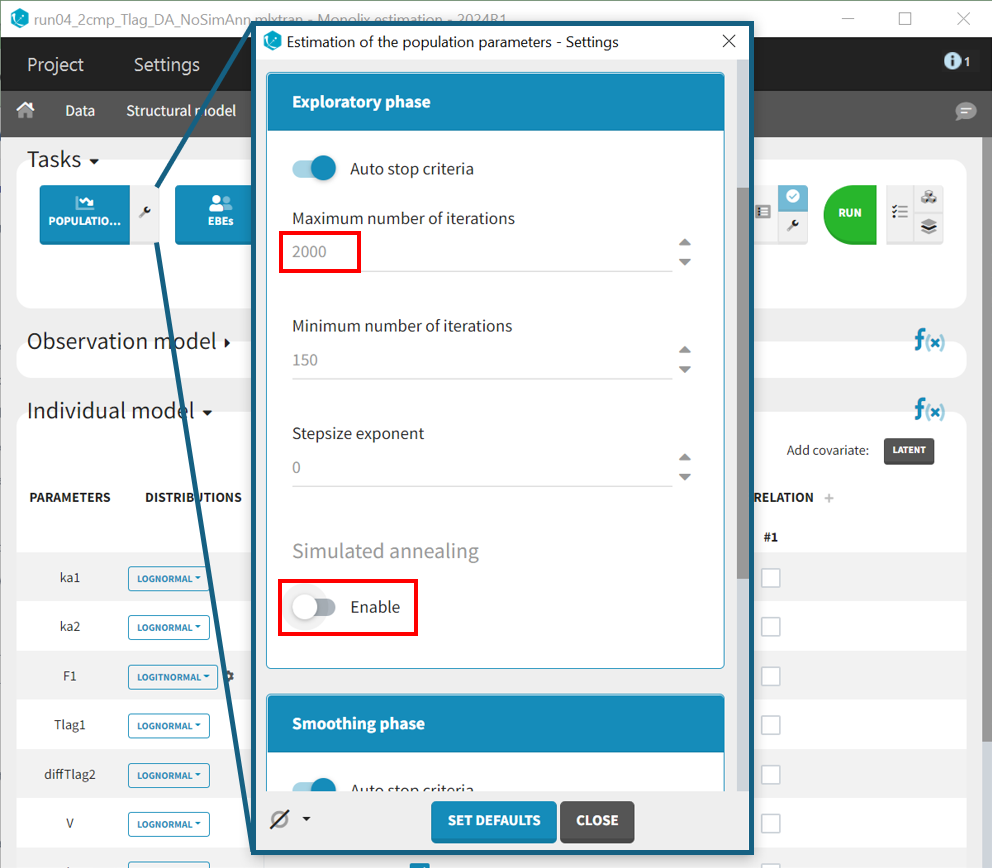
In this case, to ensure convergence, the maximum number of iterations in the exploration phase is increased from 500 to 2000, alongside disabling the simulated annealing in the settings. After making these adjustments, the project is saved under a new name (run04_2cmp_Tlag_DA_NoSimAnn.mlxtran), and all tasks are run. The results show very high R.S.E.s for and the constant error parameter . These parameters are difficult to estimate and introduce significant uncertainty into the model.

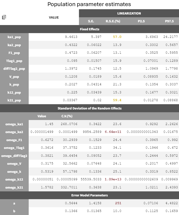
Since the omega values are nearly zero, removing them from the individual model is the next step in refining the model. As a method for parameters without variability during the population parameter estimation the default option 'No Variability' is kept and the option to enable simulated anealing is enabled again.

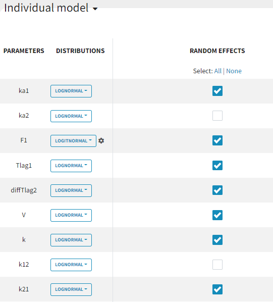
The project is saved under a new name (run05_2cmp_Tlag_DA_NoSimAnn_noEtaka2k12_NoVar.mlxtran), and all estimation tasks are run.

The parameters show reasonable estimates with borderline low R.S.E.s

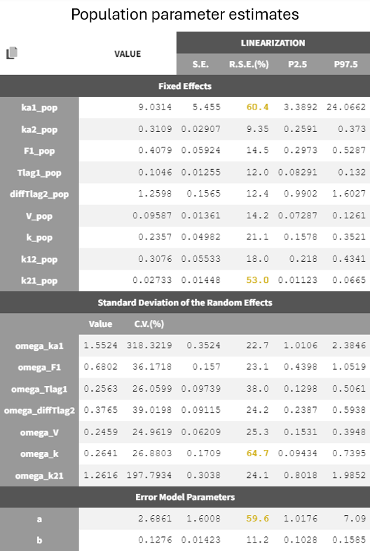
Adjustment to the residual error model

The estimation of the error parameter still shows uncertainty. In the correlation matrix of the 'Std.errors' sub-tab in the results tab, the error parameters and have the most significant correlation coefficient difference from zero (-0,7247), which could suggest that parameter may not be identifiable. Additionally, in the 'Proposal' tab of the results, it's suggested to switch to the combined 2 error model, as it provides the best fit according to the criteria. This change may improve the certainty of the parameter estimation (run08_2cmp_Tlag_DA_NoEtaka2k12_NoVar_Comb2Err.mlxtran).

The adjustment of the error model improved the fit and resulted in lower RSEs for the error parameter estimate.

run05_2cmp_Tlag_DA_NoSimAnn_noEtaka2k12_NoVar.mlxtran	run08_2cmp_Tlag_DA_NoEtaka2k12_NoVar_Comb2Err.mlxtran

Integrating correlations and assessing estimate robustness

The next evaluation step involves a closer examination of diagnostic plots and statistical tests. Enabling the information toggle in the "correlation between random effects" plot displays the correlation coefficients in the scatterplots. The scatterplot of vs suggests a correlation, with a coefficient clearly different from 0 and a noticeable incline in the regression line.

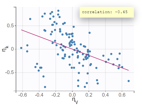
This relationship between random effects is confirmed in the statistical tests section of the results tab, where and show a significant p-value in the test for random effects correlation.

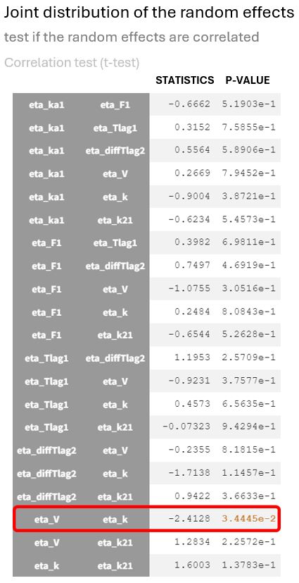
The correlation coefficient of -0.45, along with the significant p-value from the t-test for correlation suggests that the variability in and is not independent; as one increases, the other tends to decrease.

Therefore, accounting for this random effect correlation in the statistical model could be beneficial for the model. (run09_2cmp_Tlag_DA_NoEtaka2k12_NoVar_Comb2Err_CorrVk.mlxtran)

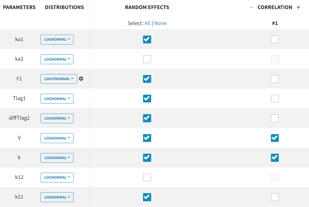
This model provides the best fit according to the information criteria -2LL (1825.4) and BICc (1902.3) throughout the entire model development process. This model adjustment also results in the fewest increased parameter estimate uncertainties, with only the R.S.E. for being slightly borderline elevated (53.1 %).

Conducting another convergence assessment with the same setup as in the section 'Assessment of parameter estimate uncertainties' (5 runs, enabling the estimation of standard errors and log likelihood with the linearization method, and sensitivity on all initial parameters) shows that the model now leads to approximately reproducible estimates with a stable log-likelihood of a maximum difference of around 1.9 points.

Predictive power of the final model

The final model was selected through a step-by-step process, alternating between model evaluation and adjustments of individual elements. The predictive power of this model is now assessed using a VPC (Visual Predictive Check), as shown below.

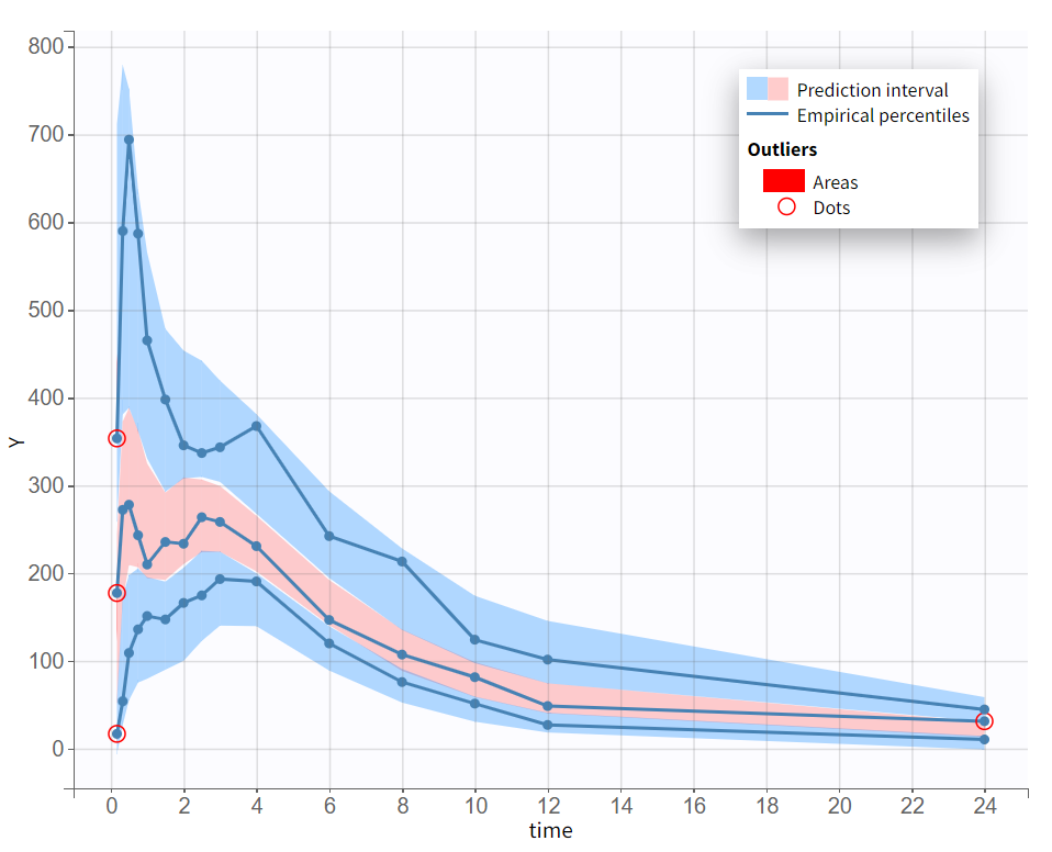
The empirical median and percentiles, represented by blue curves, align well with the predicted median and percentiles, shown as pink and blue areas. The model simulations successfully capture both the central trend, including the double peak, and the dataset variability.

In conclusion, a Monolix model was built step-by-step, effectively capturing the double peaks in the PK of veralipride.

Double absorption site model

This section applies and evaluates a model from the literature, published in:

Godfrey, KR, Arundel, PA, Dong, Z, Bryant, R (2011). Modelling the Double Peak Phenomenon in pharmacokinetics. Comput Methods Programs Biomed, 104, 2:62-9.

It is based on an approach aimed at ensuring a clear physiological interpretation. Site-specific absorption has been proposed as the key mechanism responsible for the multiple peaks observed with veralipride, where rapid absorption occurs in the proximal gastrointestinal tract, followed by a second absorption phase in more distal regions. The model describes two absorption sites with a discontinuous drug input rate, as shown below (figures from (Godfrey et al.,  2011)).

Absorption occurs at two successive sites, defined as two time windows where a constant drug input rate u(t) is applied. An identical absorption rate is assumed for both windows. Defining each time phase precisely adds complexity to the model, which requires a total of 10 parameters.

Two implementations of this model are presented: one using ODEs and another using PK macros.

Model writing with macros and ODEs

The structural model can be written with PK macros by modeling the constant input rate as two zero-order absorptions in a compartment representing the gut. The drug amount is divided between these two absorptions, with F1 representing the fraction absorbed at the first site. A transfer macro encodes the identical absorption from both sites to the central compartment.

The model file is shown below, and it is easy to read with only seven macros. Detailed documentation is available for the compartment, elimination, peripheral, absorption, and transfer macros.

[LONGITUDINAL]
input={V, ka, k, k12, k21, T1, dT1, T2, dT2, F1}

EQUATION:
odeType=stiff

PK:
; Define central and peripheral compartment
compartment(cmt=1, volume=V, concentration=Cc)
elimination(cmt=1, k)
peripheral(k12,k21)

; Define gut compartment with two zero-order inputs
compartment(cmt=3, amount=Ag)
absorption(cmt=3,Tlag=T1, Tk0=dT1, p=F1)
absorption(cmt=3, Tlag=T1+dT1+T2, Tk0=dT2, p=1-F1)

; Absorption of drug from gut compartment
transfer(from=3,to=1,kt=ka)

OUTPUT:
output={Cc}

Several Remarks:

• In the original publication, the parameter T2 represents the start of the second absorption phase. Here, T2 represents the time between the end of the first absorption and the beginning of the second, ensuring no overlap between the two absorption phases.

• The transfer rates U1 and U2 from the publication are not explicitly included. Instead, the zero-order absorptions defined with the absorption macro use the transfer duration and the fraction of the dose for each phase. However, the transfer rates can be calculated using the equations: U1=amtDose(1-F1)/dT1 and U2=amtDose(1-F1)/dT2, where amtDoseis the administered drug amount.

• PK macros offer the benefit of using analytical solutions when available. In this case, due to the transfer between the gut and the central compartment, no analytical solution is available. Therefore, the system must be solved by numerical integration. It is important to use the setting odeType=stiff to ensure a stable integration process, especially for systems that may exhibit rapid changes in dynamics.

The same model can be written using ODEs, as illustrated below. This model includes four ODEs for Ad, Ag, Ac, and Ap, which represent the drug amounts in the depot compartment, the gut, the central compartment, and the peripheral compartment, respectively. These ODEs are connected to the drug administration information using amtDose, a keyword recognized by Mlxtran to represent the administered drug amount (see all dose-related keywords). A zero-order transfer occurs between Ad and Ag, representing the drug transfer to the gut, with time-dependence handled via if/else statements. Since the zero-order transfer does not rely on system variables, the Ad variable is technically optional in this model. However, keeping it provides insight into the drug's consumption over time.

[LONGITUDINAL]
input={V, ka, k, k12, k21, T1, dT1, T2, dT2, F1}

EQUATION:
odeType=stiff

t_0 = 0
Ag_0 = 0
Ac_0 = 0
Ap_0 = 0
Ad_0 =amtDose

U1=amtDose*F1/dT1
U2=amtDose*(1-F1)/dT2

if t<=T1 ; No absorption (pre-first absorption phase)
  u=0
elseif t<=T1+dT1 ; First absorption phase, with a constant rate U1
  u=U1
elseif t<=T1+dT1+T2 ; No absorption (inter-absorption phase)
  u=0
elseif t<=T1+dT1+T2+dT2 ; Second absorption phase, with a constant rate U2.
  u=U2
else ; No further absorption occurs 
  u=0
end

ddt_Ad = -u
ddt_Ag = -ka*Ag+u
ddt_Ac = ka*Ag-(k+k12)*Ac+k21*Ap
ddt_Ap = k12*Ac-k21*Ap

Cc=Ac/V

OUTPUT:
output={Cc}

Remark:

• The model uses conditional statements to switch between absorption phases. This approach ensures that absorption from the two different sites is modeled distinctly, with the transitions between phases controlled by the conditions set on time.

Model exploration with Simulx

The exploration tab of Simulx is an application dedicated to visual exploration of model behavior, allowing easy assessment of parameter influence.

In Simulx, both models can be written simultaneously. This is useful for verifying the equivalence of different model implementations. Additionally, intermediate output vectors, beyond the concentration prediction curve Cc, can be defined and plotted to check each model component. The ability to display any model variable provides valuable simulations to understand how the model behaves.

To do this, a new Simulx project is created. In the “Definition” tab, both models are written into the model file, with minor adjustments made to the ODE-based model. The ODE equation variables and their corresponding initial conditions are indexed with "2" to distinguish them from the variables of the macro-based model. The parameter names remain the same.

[LONGITUDINAL]
input={V, ka, k, k12, k21, T1, dT1, T2, dT2, F1}

PK:
; Macro based model
compartment(cmt=1, volume=V, concentration=Cc)
elimination(cmt=1, k)
peripheral(k12,k21)
compartment(cmt=3, amount=Ag)
absorption(cmt=3,Tlag=T1, Tk0=dT1, p=F1)
absorption(cmt=3, Tlag=T1+dT1+T2, Tk0=dT2, p=1-F1)
transfer(from=3,to=1,kt=ka)

EQUATION:
odeType=stiff
; ODE based model
t_0 = 0
Ag2_0 = 0
Ac2_0 = 0
Ap2_0 = 0
Ad_0 =amtDose

U1=amtDose*F1/dT1
U2=amtDose*(1-F1)/dT2

if t<=T1 
  u=0
elseif t<=T1+dT1 
  u=U1
elseif t<=T1+dT1+T2 
  u=0
elseif t<=T1+dT1+T2+dT2 
  u=U2
else 
  u=0
end

ddt_Ad2 = -u
ddt_Ag2 = -ka*Ag2+u
ddt_Ac2 = ka*Ag2-(k+k12)*Ac2+k21*Ap2
ddt_Ap2 = k12*Ac2-k21*Ap2

Cc2=Ac2/V
OUTPUT:
output = {Cc,Cc2}

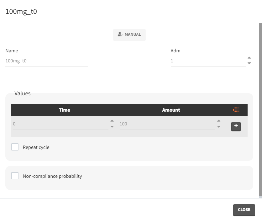
In the “Treatment” sub-tab the treatment must also be redefined, with the original regimen consisting of a single 100 mg dose administered at time 0.

Lastly, intermediary output vectors for the equation system variables (such as Ag, Ad, Ap, and u) are defined.

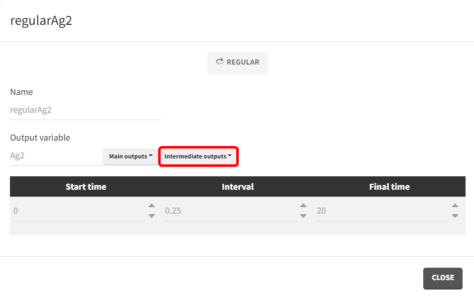
For the model written with macros, it is possible to output the drug amount in the gut and the concentration in the central compartment. However, the depot compartment is defined implicitly, and its value is not available.

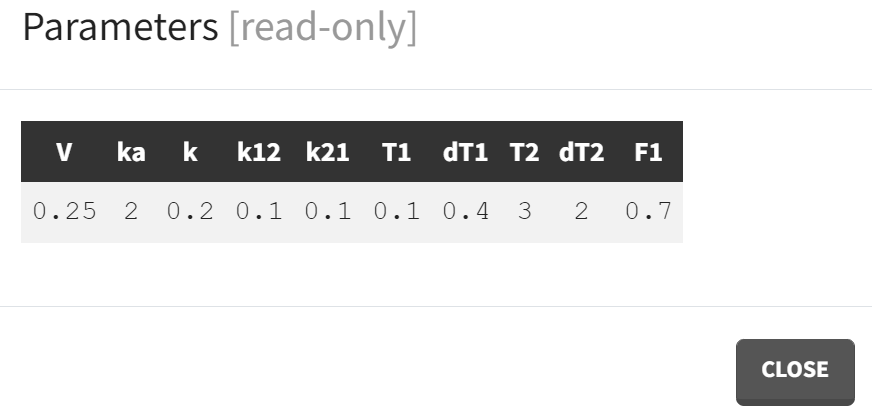
Finally, a set of parameter values is defined in the 'Parameters' sub-tab, which then dictates the prediction curves of the different output vectors for both models. The parameters have been set as follows:

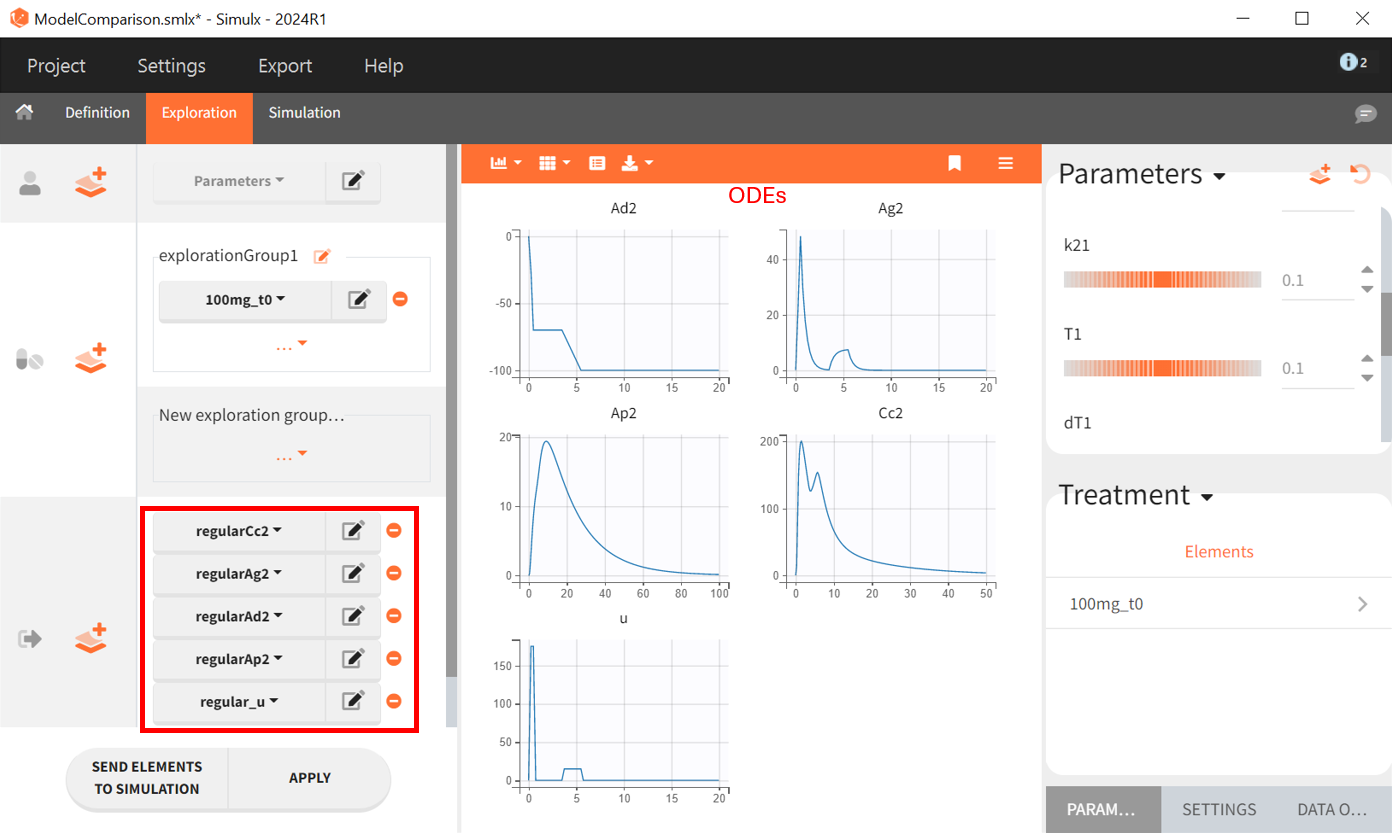
Below are the results of simulations for each model in the Exploration tab of Simulx, using the same parameter values. In the left panel, the scenario is defined. The parameters set under the object "Parameter" are those that have been specified. Within the treatment object, the treatment schedule outlines the administered therapy. The output vectors selected include the prediction curve Cc​ and the gut concentration Ag from the macro-based model, along with the corresponding output vectors Cc2 and Ag2​ from the ODE-based model.

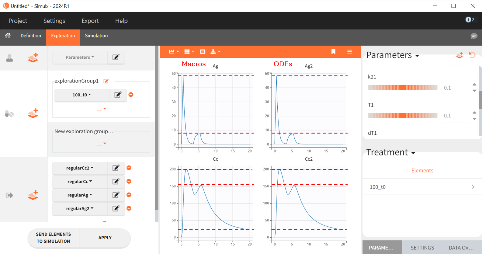
Both models generate identical prediction curves, confirming their equivalence.

In the ODE based model the amounts of drug in each compartment had to be explicitly defined. Therefore it is possible to plot them as outputs, as well as the input rate . This permits a graphical visualization of each system variable over time:

Model estimation and diagnosis with Monolix

Since both models have been verified as equivalent, either can be used in Monolix. A step-by-step modeling workflow is recommended, using the final estimates from each step as initial values for the next:

• project_1.mlxtran: A preliminary fit with only one absorption zone. Fix all parameters for the second site, and, as well as to 1 and remove inter-individual variability. Suitable initial estimates for fixed effects are required, e.g. and .

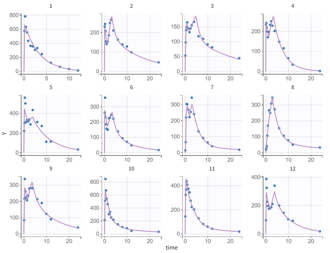
• project_2.mlxtran: All parameters are then unfixed, with a logit-normal distribution for . The estimated fixed effects of the population parameters are used as initial values, except for , which is re-initialized to 5 and its omega is set to 0.1. This preventsfrom converging to a nearby local minimum. A new estimation with SAEM is conducted. The individual fits demonstrate the model’s ability to capture double peaks. Unlike the model in section Model with two first-order absorptions, finite absorption sites allow the prediction of sharp peaks.

However, the parameters and show elevated R.S.E.s (73.3, 51.8). The parameters and also exhibit increased R.S.E.s (62.8, 140). Additionally, conducting a convergence assessment reveals a significant variation in the log-likelihood between runs, with a range difference exceeding 40 points.

• project_3.mlxtran: since the estimates should now be close to the global solution, the simulated annealing option can be disabled in the settings of SAEM. To ensure convergence, the maximum number of iterations in the exploration phase is increased from 500 to 2000. After running again, the parameter converged very close to zero during the estimation task with very high R.S.E (3.91e+7). Removing the random effect ofmight be beneficial to the model.

• project_4.mlxtran: As a method for estimating parameters without variability, the option "Add decreasing variability" is selected in the SAEM settings. This method adds artificial variability (random effects) to parameters for SAEM estimation, starting at omega=1 and decreasing exponentially to 1e-5 by the end of the process, based on maximum iterations in exploratory and smoothing phases.
  The estimates have been assessed with good to slightly borderline certainty.
  Except for the random effect of , the R.S.E.s of estimates are within a reasonable range. However, the R.S.E. for remains unacceptably high, indicating the need for further model adjustments. Variability for is removed, and a new model run is conducted.

• project_5.mlxtran: Several parameters show increased R.S.E.s, suggesting model over-parameterization, as adjustments to one parameter have influenced the estimates of others. To address this, the variance-covariance matrix is recalculated, now using stochastic approximation instead of linearization. To ensure calculation of the Fisher Information Matrix, the maximum number of iterations in the standard error task is increased from 200 to 500. Significant non-zero correlation coefficients related to are observed, including = -0.8434 and = 0.8325. For the next run, parameter is fixed to reduce interdependencies.

• project_6.mlxtran: Overall estimates show good to slightly borderline certainty. Re-running the standard error task with stochastic approximation reveals no correlations for parameters , and with other parameters, though some elevated correlations persist among other parameter pairs. A potential model improvement could involve changing the error model from combined 1 to combined 2.

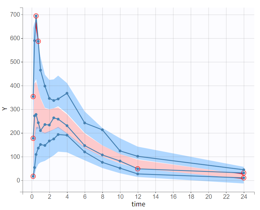
• project_7.mlxtran: Overall, the model provides acceptable parameter estimates with good to borderline certainty. A convergence assessment with sensitivity to initial values indicates a log-likelihood difference of 10 points due to model adjustments, reflecting significant stability improvement over project_2.mlxtran.

Diagnostic plots confirm that the model captures the data's characteristics well, and the VPC demonstrates good power.

Compared to project_2.mlxtran, project_7.mlxtran has slightly better information criteria; however, reliance on the log-likelihood should be cautious as both monolix prjects yield unstable estimates. Although project_7.mlxtran’s BICc reduction of approximately 11.4 points is significant, this is likely due to parameter removal.

project_2.mlxtran	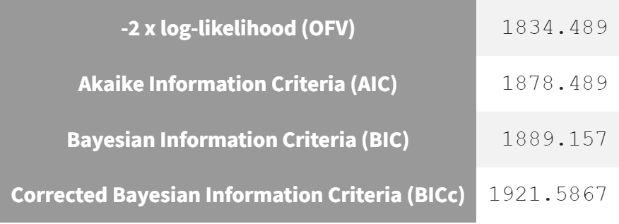project_7.mlxtran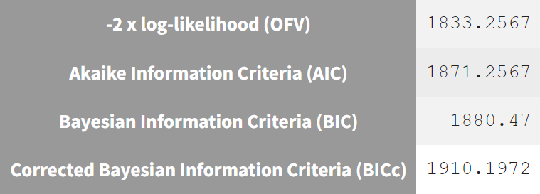

Both models, parallel absorption model and site-specific absorption model, capture the primary data behavior well, yet the final model from section “Modeling parallel absorption processes“ provides stable estimates and will therefore serve as the basis for the next section, where new scenario simulations will be conducted.

Simulations and model validation

The simulations will be conducted in Simulx, using both its interface and the lixoftConnectors package in R, which offers integration with MonolixSuite.
In the simulations chapter, the therapeutic window is explored by tracking how long drug concentrations remain above a target level, which provides insights into the consistency and effectiveness of therapeutic exposure across individuals. This analysis helps determine if the drug concentration remains within an effective range. Additionally, AUC is analyzed for each subject to assess exposure variability across the population, with subjects divided into quartiles (lowest 25%, 2nd, 3rd, and highest 25%) to reveal differences in drug concentrations. This approach uncovers patterns often missed by overall averages.

The final model estimated in section “Modeling parallel absorption processes“, involving parallel first-order absorption, will be used to simulate drug effects on a large population. Simulx enables flexible simulations by reusing all Monolix project elements, such as model, estimated parameters, and dataset design, while allowing adjustments to parameters or design as needed. Here, the number of individuals and outputs will be modified to display the AUC and the therapeutic window duration.

Simulations with Simulx

Before running the simulations, the final project must be exported from Monolix to Simulx.

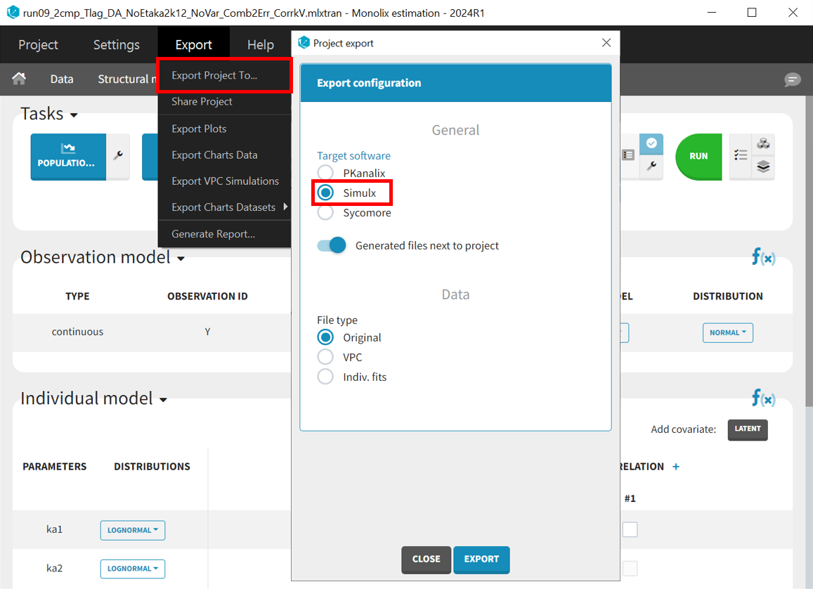
All the information contained in the Monolix project will be transferred to Simulx. This includes the model (longitudinal and statistical part), the estimated population parameter values and their uncertainty distribution and the original design of the dataset used in Monolix (number of individuals, treatments, observation times). Elements containing these information are generated automatically in the “Definition” tab of the created Simulx project. It is possible to reuse these elements to setup a simulation in the “Simulation” tab or create new elements to define a new simulation scenario.

For the new simulation scenario, the AUC under the prediction curve ​ will be calculated directly within the model file. To do this, click "Add additional lines" and insert these two lines of code:

AUC_Cc_0=0
ddt_AUC_Cc=Cc

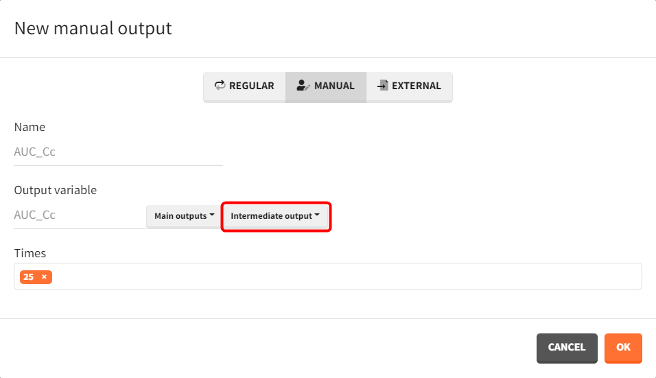
A corresponding output vector is defined to capture each subject’s AUC value at 25 hours.

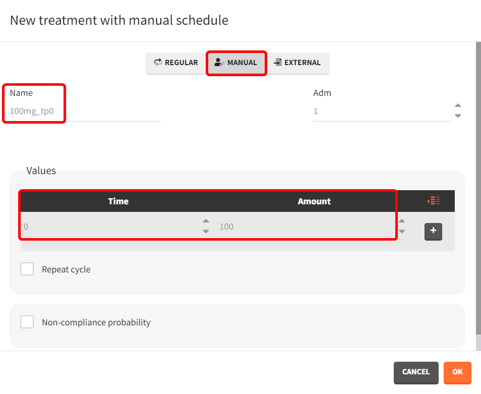
To simulate more subjects than in the original dataset, the dose and schedule need to be modified in the "Treatment" sub-tab of the "Definition" tab. Click the plus sign, set the administration time to 0, and enter 100 mg as the amount, naming the elemnt "100mg_tp0."

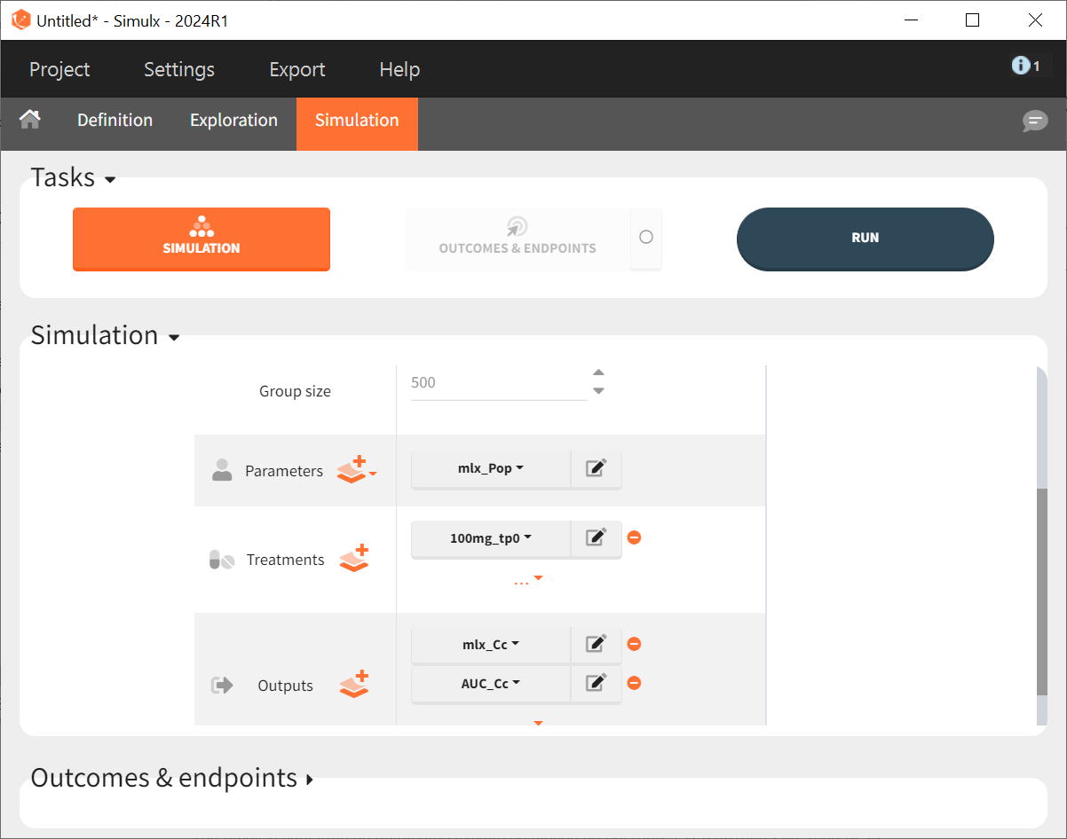
In the "Simulations" tab, adjust Group size from 12 to 500, select "100mg_tp0" as the treatment, and choose "mlx_Cc" and "AUC_Cc" as outputs. Keep "mlx_Pop" for the parameter vector, as it reflects the final population parameters from the Monolix project.

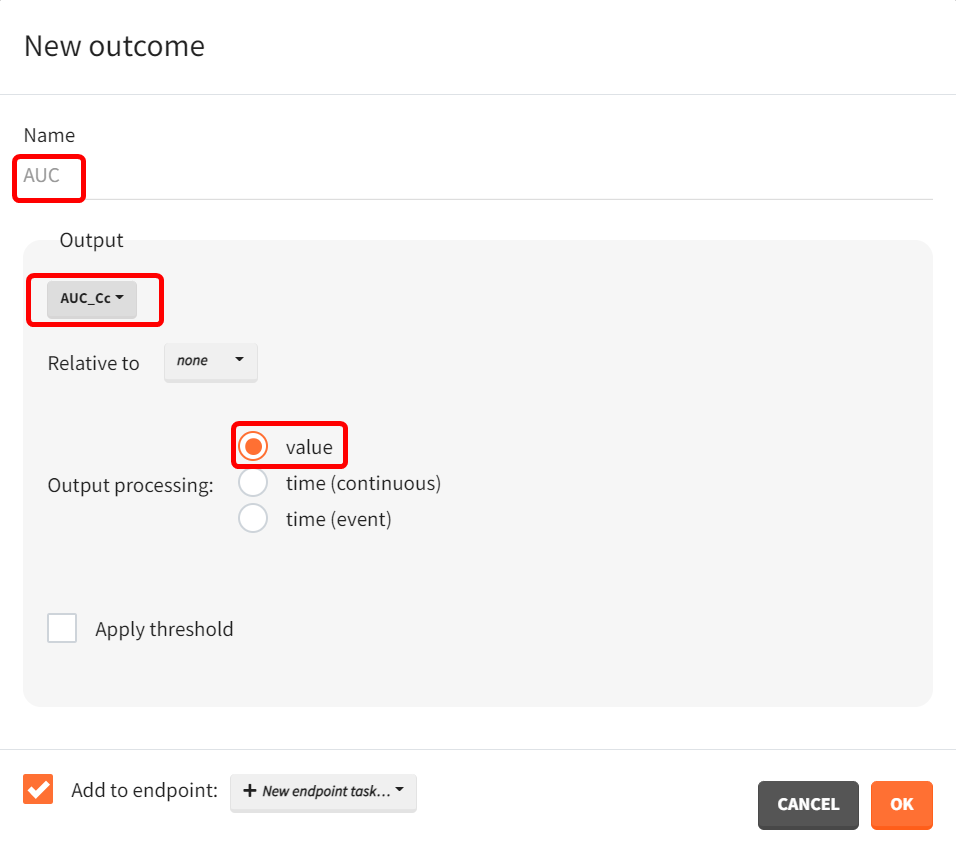
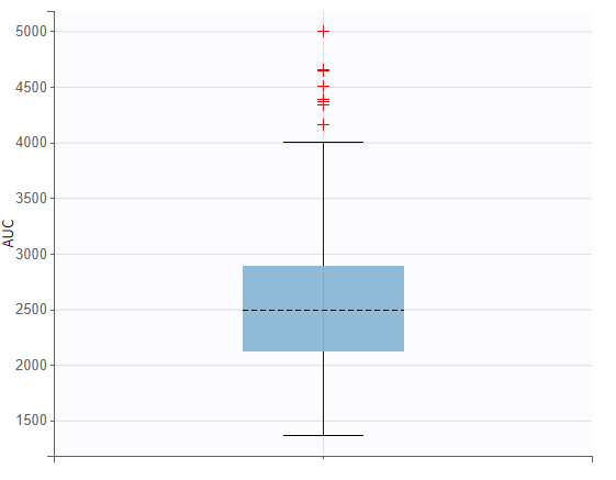
The setup for displaying simulation results is specified in the “Outcomes & endpoints“ panel. For “AUC_Cc”, the values for all subjects shall be summarized and presented as a distribution in form a boxplot or pdf. “AUC” is chosen as the outcome name, based on the “AUC_Cc” output vector, and "value selected" is kept for output processing.

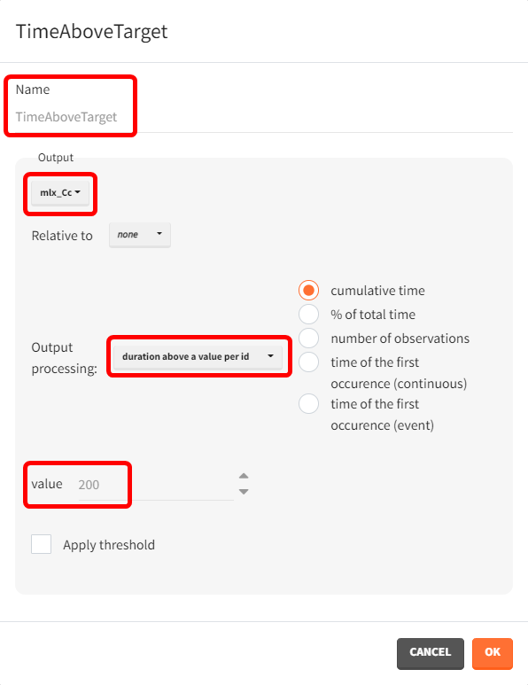
For the therapeutic window, the time during which the concentration remains above the target of 200 ng/mL is calculated. This outcome is named TimeAboveTarget, based on the concentrations output vector. "Duration above a value per ID" is selected for output processing to capture the cumulative time above 200 ng/mL, providing a continuous measure. This cumulative approach accommodates the double-peak absorption model, where some subjects may exceed the target value twice.

Another outcome is defined here, similar to the TimeAboveTarget outcome. In this case, a logical operator and a threshold are added to evaluate how many subjects had a cumulative time above the target of 200 ng/mL for 2 hours or more. This is done by duplicating the TimeAboveTarget outcome definition and enabling the "Apply threshold" checkbox. This action activates a dropdown menu and a field to select the operator and set the value to 2. The outcome name is also updated accordingly.

This outcome will not be continuous but rather a Boolean result, indicating both the percentage and total number of subjects (out of 500) who met this criterion.

With these definitions, the simulation can be conducted, capturing the specified outcomes and endpoints.

Evaluating the results and plots reveals that the 500 resampled subjects spend an average of 4.18 hours above the target concentration, with a standard deviation of 1.7 hours. This is illustrated in two ways: first, by the “Cc output distribution” plot with a visual cue at y=200 to indicate the target, and second, by the “TimeAboveTarget” outcome distribution plot, which summarizes the time above 200 ng/mL as a boxplot.

Cc - Output distribution	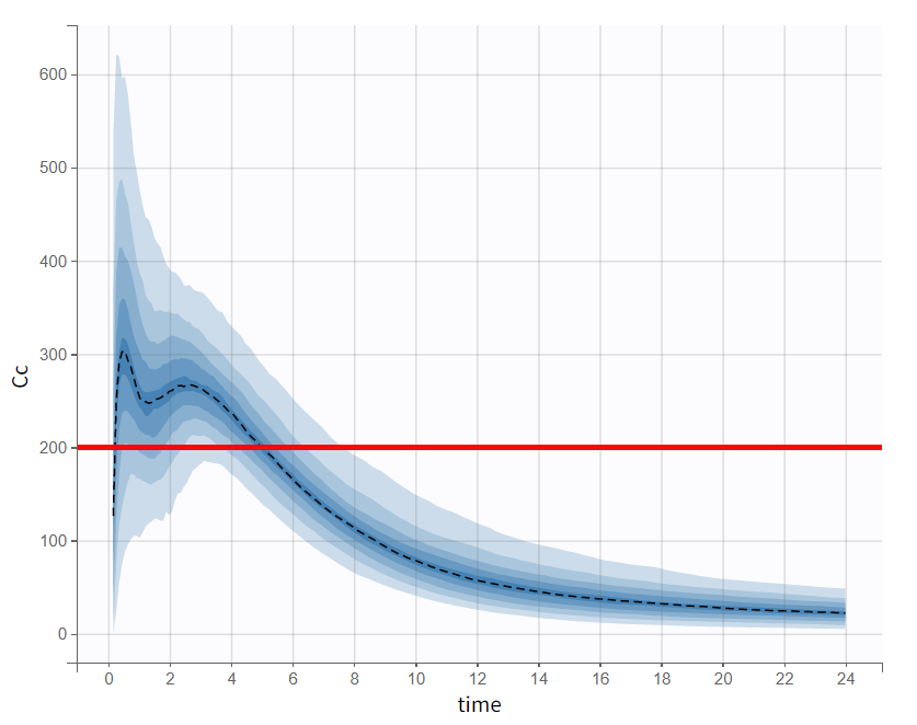TimeAboveTarget - Outcome distribution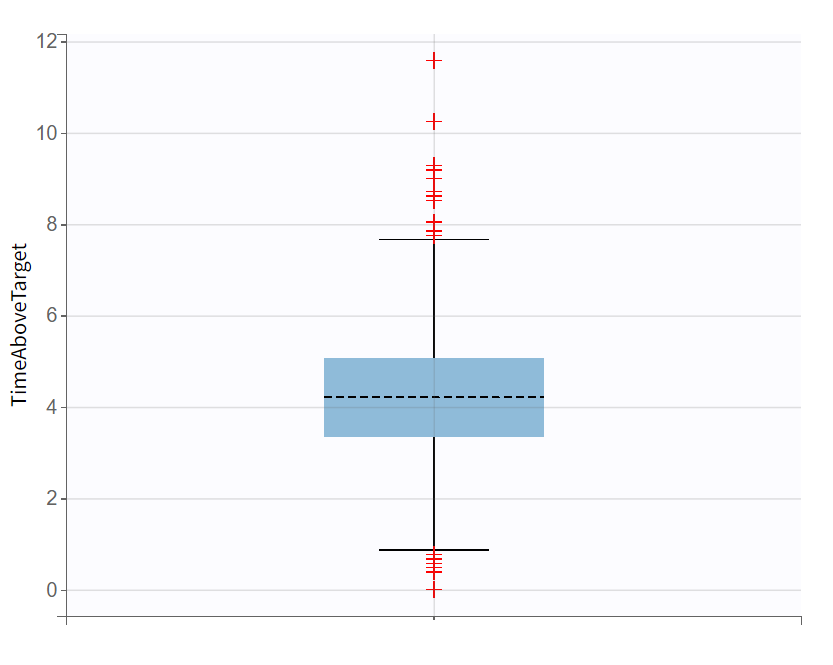

The area under the concentration prediction curve, aggregated across all 500 subjects, is also be visualized as a boxplot.

The simulations performed in the Simulx interface can also be conducted in R using the lixoftConnectors package.

Simulations and post processing with lixoftConnectors

Steps for setting up the simulation scenario follow the chronological order as performed in the interface.

# GOAL: Assessing AUC and therapeutic window through simulation
# loading the lixoftConnectors library
library(lixoftConnectors)
path.software <- paste0("C:/Program Files/Lixoft/MonolixSuite2024R1") 

# software initialization: specify the software to be used
initializeLixoftConnectors(path.software,software = "monolix")
options(lixoft_notificationOptions=list(errors=0, warnings=1, info=1))

# loading the final Monolix project
name.project <- "run09_2cmp_Tlag_DA_NoEtaka2k12_NoVar_Comb2Err_CorrkV.mlxtran" 
path.project <- paste0(file.path(dirname(path.prog),"2_double_oral_absorption"),"/",name.project)
loadProject(projectFile = path.project)

# export monolix project to simulx
exportProject(settings = list(targetSoftware = "simulx", filesNextToProject = T), force=T)

# add lines ot calculate AUC_Cc
setAddLines(
"AUC_Cc_0 = 0
ddt_AUC_Cc = Cc")

# define output vector for exposure parameter AUC_Cc
defineOutputElement(name = "AUC_Cc", element = list(data = data.frame(time=25), output="AUC_Cc"))

# define treatment: 100mg at time point 0
defineTreatmentElement(name = "100mg_tp0", element = list(data=data.frame(time=0, amount=100)))

# set simulation scenario
setGroupElement(group = "simulationGroup1", elements = c("mlx_Pop", c("mlx_Cc", "AUC_Cc"), "100mg_tp0"))
setGroupSize("simulationGroup1",500)

# define time above target as outcome
defineOutcome(name = "TimeAboveTarget",    element = list(output = "mlx_Cc", processing = list(operator = "durationAbove", type = "cumulativeTime", value = 200)))
defineOutcome(name = "TimeAboveTarget_2h", element = list(output = "mlx_Cc", processing = list(operator = "durationAbove", type = "cumulativeTime", value = 200), applyThreshold=list(operator= ">=", value=2)))

# define endpoints 
defineEndpoint(name = "TagetWindow",    element = list(outcome = "TimeAboveTarget",    metric = "arithmeticMean"))
defineEndpoint(name = "TagetWindow_2h", element = list(outcome = "TimeAboveTarget_2h", metric = "percentTrue"))

# set calculation of both simulation and endpoints
setScenario(c(simulation = T, endpoints = T))
runScenario()

Note that AUC was not defined as an outcome here. This step was only required in the interface so that AUC could be plotted as a boxplot (or alternatively as pdf, cdf).

Afterward, results need only be retrieved via the connectors getEndpointsResults() and getSimulationResults() and converted into an appropriate format, enabling plot creation with the ggplot. package.

# retrieve results
res_AUC <- data.frame(id     = getSimulationResults()$res$AUC_Cc$id,
                      metric = c("AUC"),
                      value  = getSimulationResults()$res$AUC_Cc$AUC_Cc)

Retrieving the data for simulated concentration profiles as well as for the time above target outcome variable works analogous. Note that has a longitudinal format, representing a time profile, unlike AUC, which consists of only a single value per subject. Therefore, the time variable also needs to be retrieved.

With the following settings, a boxplot can be created that is very similar to the one in the interface. However, it is not necessary to specify so many settings if the boxplot does not need to look as refined.

# Load ggplot2
library(ggplot2)

# create the boxplot for AUC
boxplot_AUC <- ggplot(res_AUC, aes(x = metric, y = value)) +
  geom_boxplot(width = 0.5, notch = FALSE, fill = "#8FBBD9", outlier.shape = 4, outlier.size = 3, outlier.color = "#FF0000", color = "#000000", fatten = NA) +  
  stat_summary(fun = mean, geom = "errorbar", width = 0.5, aes(ymax = ..y..,ymin = ..y..), color = "#000000", linetype = "dashed", size = 0.5, show.legend = FALSE) +
  labs(y = "AUC", x="") +
  scale_x_discrete(labels = NULL)

The following boxplot display is obtained:

AUC - Outcome distribution	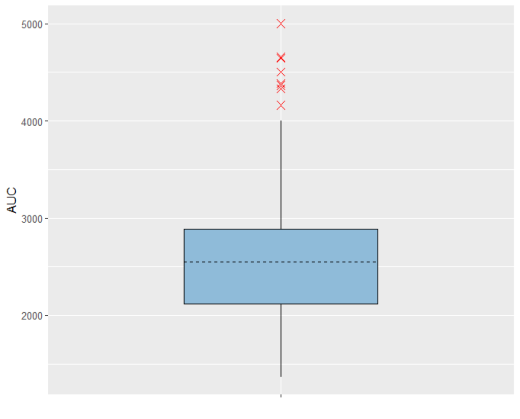TimeAboveTarget - Outcome distribution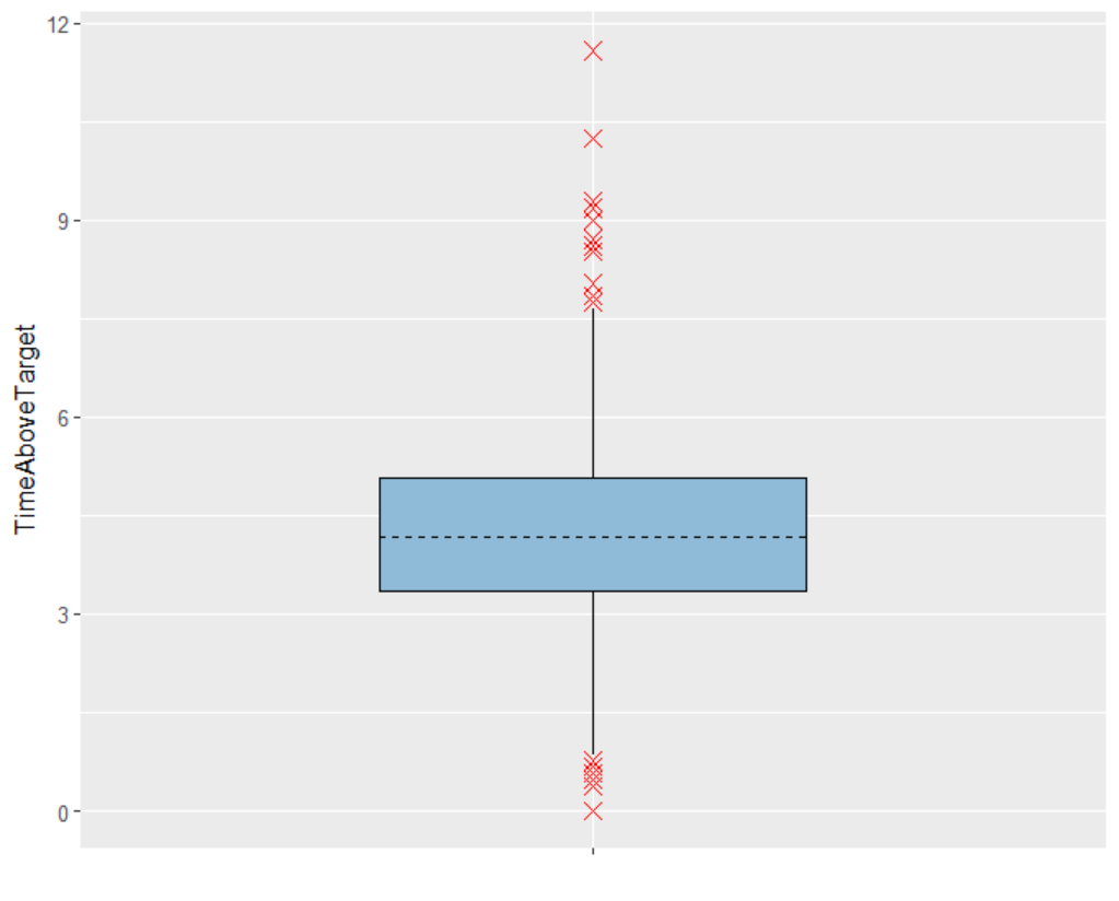

To create the output predictions plot, some data manipulation is required. The concentration percentiles over time must be calculated.

# load ggplot2
library(dplyr)

# calculate median and percentiles by time
res_Cc_summary <- res_Cc %>%
  group_by(time) %>%
  summarize(median = median(value),
            p10    = quantile(value, 0.1),
            p20    = quantile(value, 0.2),
            p30    = quantile(value, 0.3),
            p40    = quantile(value, 0.4),
            p50    = quantile(value, 0.5),
            p60    = quantile(value, 0.6),
            p70    = quantile(value, 0.7),
            p80    = quantile(value, 0.8),
            p90    = quantile(value, 0.9))

After the dataframe contains the percentile information, the output distribution plot can be generated.

# Plot the median and percentile bands
outputdistrib_Cc <- ggplot(res_Cc_summary, aes(x = time)) +
  geom_ribbon(aes(ymin = p10, ymax = p90), fill = "#B3CDE3", alpha = 0.4) +
  geom_ribbon(aes(ymin = p20, ymax = p80), fill = "#8FBBD9", alpha = 0.4) +
  geom_ribbon(aes(ymin = p30, ymax = p70), fill = "#66A5D9", alpha = 0.4) +
  geom_ribbon(aes(ymin = p40, ymax = p60), fill = "#4199D9", alpha = 0.4) +
  geom_line(aes(y = median), color = "#553DA2", size = 0.1) +
  geom_hline(yintercept = 200, color = "#FF0000", linetype = "solid") +  
  labs(x = "time", y = "Cc")

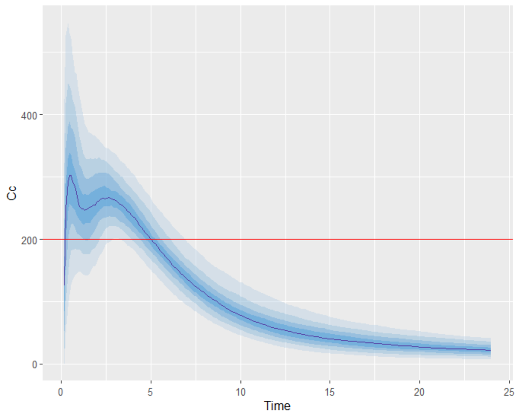
Through some post-processing of the result data, the time-above-target outcome can be represented as a histogram. Additionally, from the endpoint getEndpointsResults()$endpoints$TargetWindow_2h, it is found that a total of 453 subjects had a cumulative time above target of 2 hours or more, which corresponds to 90.6% of the simulated population.

# Create a histogram for TimeAboveTarget values
histogram_TAT <- ggplot(res_TimeAboveTarget, aes(x = value)) +
  geom_histogram(binwidth = 0.50, fill = "#8FBBD9", color = "black", alpha = 0.7) +
  geom_vline(xintercept = 2, color = "#FF0000", linetype = "solid") +
  stat_bin(binwidth = 0.50, aes(label = ..count..), geom = "text", vjust = -0.5, size = 2) +
  labs(x = "Time above target", y = "Number of Subjects per bin") 

Conclusion

This case study compared two distinct modeling approaches:

The first approach, considering a parallel absorption process, involved developing a model in Monolix with a step-by-step workflow, alternating between model evaluation and individual adjustments. No over-parameterization issues were identified. Instead, a correlation between random effects was observed and addressed. Convergence assessment confirmed very stable estimates and log-likelihood values, supporting model reliability.

In the second approach, a model with two successive absorption windows was implemented twice—once using PK macros and once using ODEs. Both implementations were verified for equivalence in Simulx’s Exploration tab before model development continued in Monolix. Although the model successfully captured key observation characteristics, it ultimately did not yield stable log-likelihood and estimate values. Given these findings, the first model was chosen for simulation purposes.

In the final phase, simulations were conducted based on the validated Monolix model, with a new scenario defined and result post-processing applied to facilitate interpretation. Simulx then provided new outputs, enabling effective evaluation of the drug's effect in a larger population.