QSP Modeling: FAAH Inhibitor Case Study

Download Materials | Download QSP model in mlxtran

This case study demonstrates application of Quantitative Systems Pharmacology (QSP) modeling in drug development, using the example of a Fatty Acid Amide Hydrolase (FAAH) inhibitor. It is a practical, step-by-step guide to build, calibrate, and use a QSP model to address key questions. It shows how to integrate various data sources—from in vitro and preclinical studies to human clinical data—to build a robust mechanistic model. This case study also explains the impact of the sensitivity analysis and uncertainty assessment, showing how these techniques can inform critical go/no-go decisions and guide future research.

https://youtu.be/kUEKwANvj2I

Introduction to QSP Models

Quantitative Systems Pharmacology (QSP) models are a powerful tool for understanding the dynamic interactions between a drug and a biological system. Unlike traditional pharmacokinetic/pharmacodynamic (PK/PD) models, which often use empirical relationships, QSP models incorporate a greater level of biological detail.

This approach positions QSP at a continuum between QSP and other approaches such as systems biology and population PK/PD. Compared to pop PK/PD, QSP usually have more biological details, that describe more chemical species than what can be measured experimentally. They can cross over different scales: tissue, organ and whole body.

One of the key challenges in QSP is that it's often not feasible to estimate every single model parameter from experimental data alone. As a result, many parameters are fixed based on existing literature or prior knowledge. This also means QSP models typically consider less inter-individual variability compared to population PK/PD models, focusing more on the core biological mechanisms.

Goals and Challenges

Summarizing biological knowledge into a mathematical framework offers several key advantages that make QSP an invaluable tool in drug development:

• Identifying Knowledge Gaps: The process of building a QSP model forces a high degree of precision, exposing gaps in our biological understanding. If a model fails to capture observed data, it signals that an important, un-modeled mechanism is at play, guiding future research.

• Checking Model Viability: A QSP model can be used to test hypotheses and determine if our current understanding is sufficient to explain experimental data.

• Answering "What-If" Questions: Complex biological systems have many redundancies and feedback loops, making it difficult to predict the effects of a new drug or intervention without a model. QSP allows for virtual simulations of new scenarios, enabling better-informed decisions.

QSP models can be applied at all stages of drug development, from target identification and biomarker evaluation to clinical trial design, patient selection, and investigating unexpected results. Ideally, the QSP model evolves alongside the drug development project, becoming more refined as new data becomes available.

Real-World Examples of QSP in Drug Development

QSP has been successfully applied to a variety of drug development challenges, as shown in these examples:

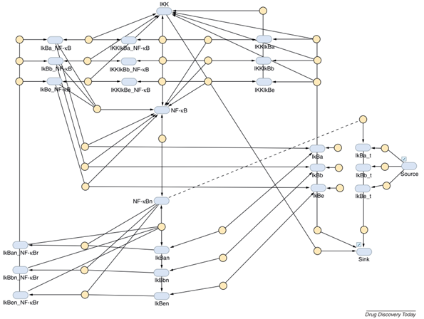
Pre-clinical: Targeting NF-kB in Chronic Obstructive Pulmonary Disease (COPD)

Cucurull-Sanchez, L., Spink, K. G., & Moschos, S. A. (2012). Relevance of systems pharmacology in drug discovery. Drug Discovery Today, 17(13–14), 665–670.

• Case: Researchers aimed to use RNA interference to modulate the inflammatory response in COPD by targeting the NF-kB pathway.

• QSP Question: What is the best target within this pathway to prevent NF-kB activation, and how much downregulation is needed to achieve the desired reduction of NF-kB nuclear translocation?

• QSP Insight: Analysis revealed that the IIK-2 kinase was the most effective target. Simulations further predicted that a 20-fold reduction in IIK-2 was necessary to achieve the desired effect. This proved to be a challenging goal, as current siRNA therapies only achieve a 5-fold reduction, highlighting a significant hurdle for the program.

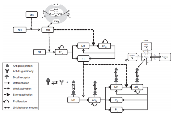
Translation from Preclinical to Clinical: Predicting Immunogenicity

Chen et al.(2014). A mechanistic, multiscale mathematical model of immunogenicity for therapeutic proteins: Part 2 - Model applications. CPT: Pharmacometrics and Systems Pharmacology, 3(9), 1–10.

• Case: Therapeutic proteins can trigger an unwanted immune response (immunogenicity). Because it highly depends on the host immune system, the response is difficult to predict in humans based on animal models.

• QSP Question: What is the predicted immunogenicity of adalimumab in a specific human population (North American, with a specific MHC-II allele frequency)?

• QSP Insight: A multiscale model incorporating antigen presentation, T-cell activation, and antibody production predicted that after 19 months of treatment, 75% of the population would be positive for anti-drug antibodies (ADA+), providing a quantitative prediction to inform clinical strategy.

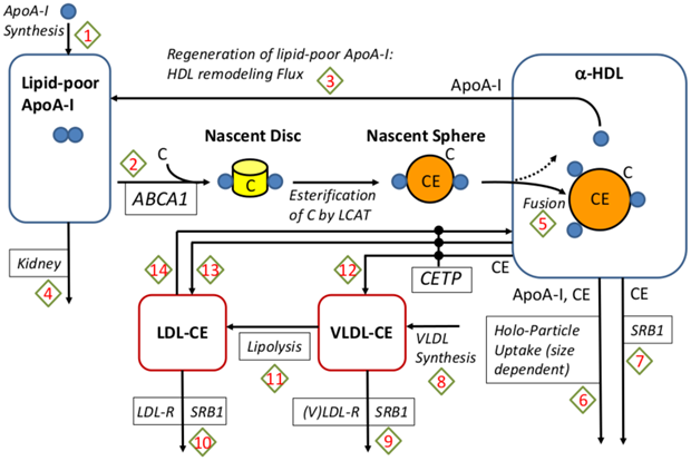
Clinical: Understanding Past Failures in Cholesterol Therapy

Example of the application of QSP models at this stage is shown in this case study in the next section.

Lu  et al. (2014). An In-Silico Model of Lipoprotein Metabolism and Kinetics for the Evaluation of Targets and Biomarkers in the Reverse Cholesterol Transport Pathway. PLoS Computational Biology, 10(3).

• Case: HDL mediates reverse cholesterol transport (RCT) and thus contributes to lower cardiovascular diseases (CVD) risk. Several therapies designed to raise HDL cholesterol, such as CEPT inhibitors, have failed to reduce cardiovascular disease (CVD) risk despite showing a strong effect on HDL levels. A QSP model has been developed to include the geometric structure of HDL. It links the core radius with the number of ApoA-I molecules on it, and the regeneration of lipid-poor ApoA-I from spherical HDL due to remodeling processes.

• QSP Question: Why did CEPT inhibition fail, and would a different target be more effective?

• QSP Insight: A detailed QSP model of lipoprotein metabolism showed that while CEPT inhibitors increased HDL, they did not change Reverse Cholesterol Transport (RCT), the key process that links HDL to a reduced CVD risk. The model demonstrated that the correlation between HDL and CVD was not causal in this context. Furthermore, the model identified ABCA-1 as a more promising target that could effectively increase RCT.

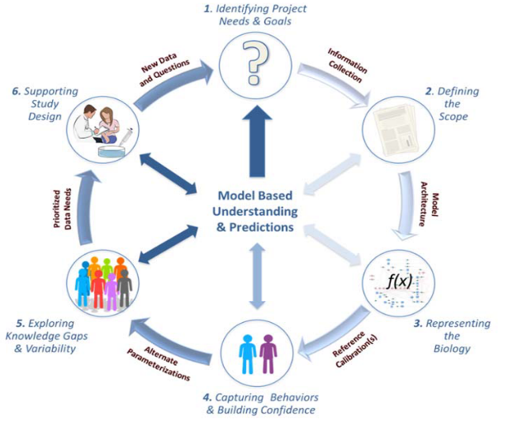
QSP Workflow

QSP modeling is a complex process. Two primary challenges are the extensive parameterization required and the computational demands of running these complex models.

A typical workflow involves several key steps, though in practice, it is often an iterative process with frequent back-and-forth between these stages.

1. Identify Project Needs and Goals: The process begins with a clear articulation of the key questions to be answered by the model.

2. Define the Model Scope: This involves specifying which biological components and scales (e.g., cellular vs. whole-body) to include, driven by the project's goals and available data.

3. Represent the Biology: The biological system is first mapped out in a conceptual diagram, followed by the translation into mathematical equations. It is crucial to document all assumptions in clear, non-technical language to facilitate communication.

4. Calibrate the Model: Parameter values are defined using a combination of literature data, experimental data, and model fitting to clinical observations. The model's behavior is then compared to available data to build confidence.

5. Explore Knowledge Gaps and Variability: The impact of uncertainties in model parameters is assessed, often through sensitivity analyses, to understand how robust the model's predictions are.

6. Support Study Design: The final, calibrated model is used to simulate new scenarios and answer the initial project questions.

Case Study: FAAH Inhibitor

This case study, based on a publication by Benson et al. (2014), examines the development of PF-04457845, an irreversible FAAH inhibitor for osteoarthritic pain.

N. Benson, E. Metelkin, O. Demin, GL. Li, D. Nichols, PH van der Graal (2014). A Systems Pharmcology Perspective on the Clinical Development of Fatty Acid Amide Hydrolase Inhibitors for Pain. CPT: Pharmacometrics Systems Pharmacology 3e91.

Data are extracted from the plots, and only the PK part of the model was changed compared to the publication.

Introduction

FAAH stands for Fatty Acid Amide Hydrolase. This enzyme degrades fatty amides such as anandamide (AEA). AEA, in turn, binds to the CB1 receptor in the brain, which decreases the perception of pain.

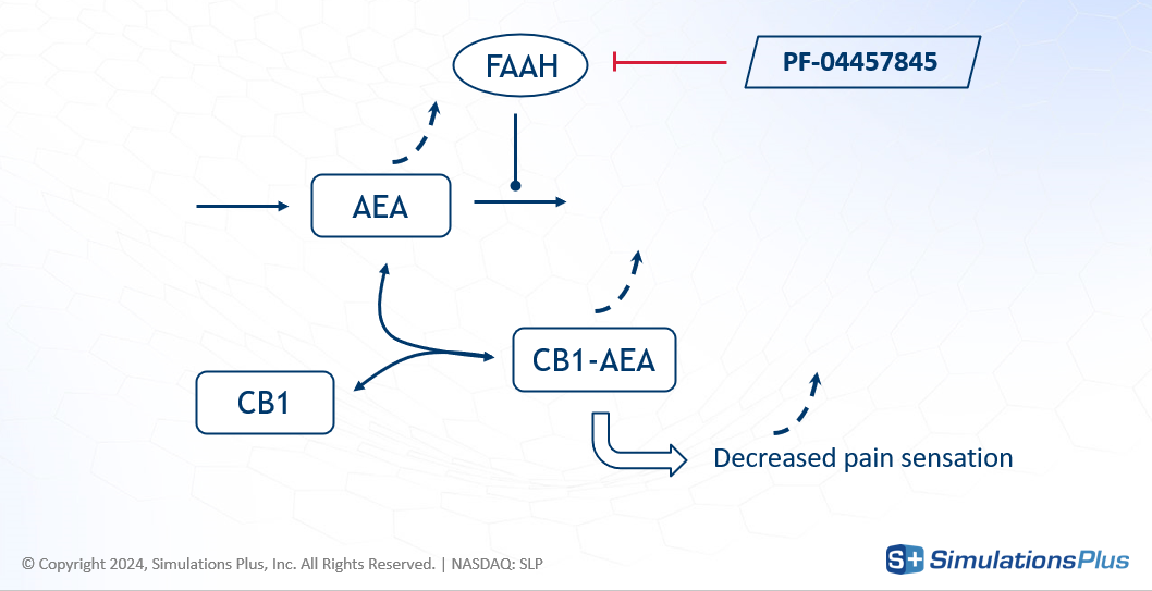
The drug of interest, PF-04457845, is an irreversible FAAH inhibitor, developed for osteoarthritic pain. By inhibiting FAAH, the drug increases AEA concentration - less degradation - leading to greater CB1 occupancy and a reduction in pain.

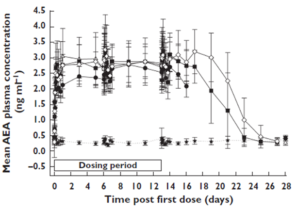
The preclinical data for this drug shows some or no effect depending on the stimulus intensity and the disease animal model, but the phase I clinical data showed a strong effect: FAAH was inhibited by over 97% in plasma

and AEA concentration increased significantly.

This led to a crucial set of questions between Phase I and Phase II:

• Is our understanding of the underlying biology sufficient to move to the next phase?

• What is the required dose to elicit a clinical effect?

The goal of this study was to develop a QSP model to capture the known biology and simulate the effect of different doses on CB1 occupancy.

Model

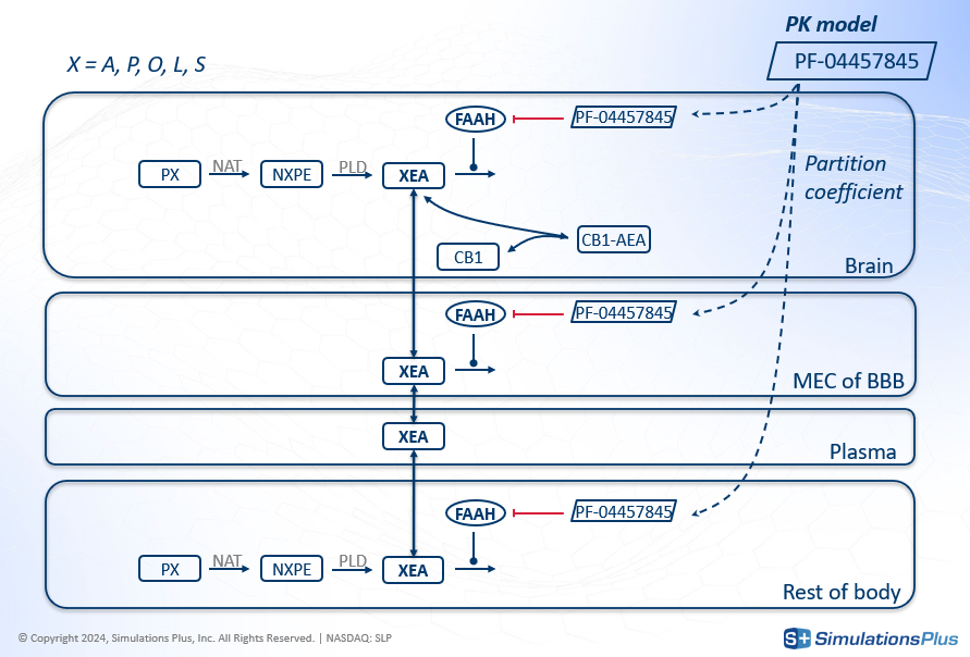
The agonist effect on CB1 happens in the brain, but FAAH is also present in other organs. So the model developed to answer these questions was a minimal PBPK (Physiologically-Based Pharmacokinetics) model that included the brain, blood-brain-barrier, plasma, and other body compartments. Key features of the model included:

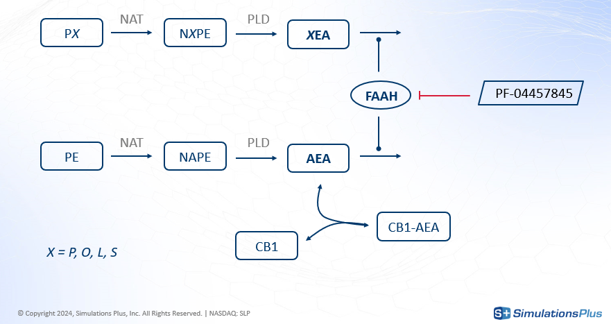
• The two-step synthesis of AEA and its degradation including PE and NAPE.

• The degradation of four different fatty amides (grouped as XEA), which compete with AEA for the FAAH enzyme.

• The transport of XEAs, including AEA, across different compartments.

• The drug's inhibition of FAAH everywhere except in the plasma.

• The concentration of drug in each compartment derived from a PK model using partition coefficients.

In total this model has 62 reactions rates, 38 ordinary differential equations (ODEs) and 96 parameters - highlighting the scale and detail typical of QSP:

• 8 PK parameters

• 15 organ volumes

• 5 molecular mass

• 8 partition coefficients

• 20 enzyme or precursor distribution

• 9 reaction velocity

• 15 Km or inhibition constants

• 6 transport rates

• 10 relative speed between XEAs.

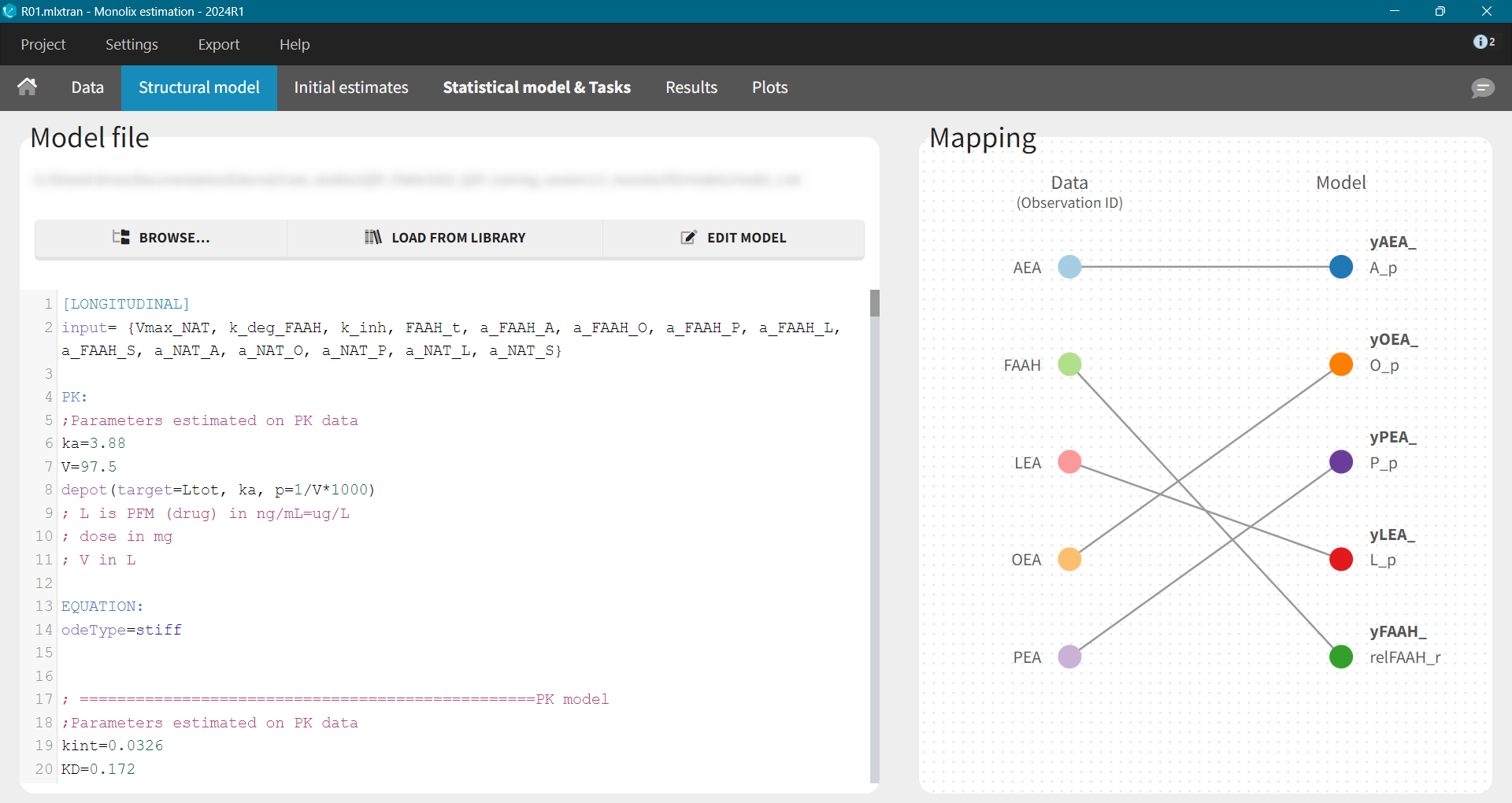
Model Implementation in Monolix

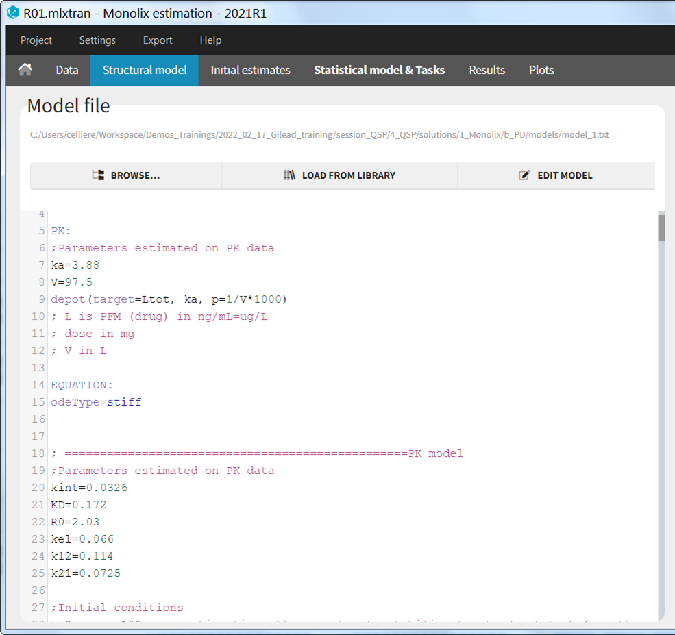
The implementation of this model in the mlxtran language - used in Monolix - required careful attention to several details:

• Input Parameters: Parameters were defined as either to be estimated or fixed from literature.

• PK Block: A depot macro was used to define how the doses present in the data set will be applied to the system. The argument target indicates to which ODE variable the dose is added.

[LONGITUDINAL]
input= {Vmax_NAT, k_deg_FAAH, k_inh, FAAH_t, ...}

PK:
depot(target=Adrug)

• ODE Solver: The odeType = stiff setting was used to switch to an implicit solver, better suited for the computational demands of QSP. Fixed parameters were defined here as well.

EQUATION:
odeType = stiff

; fixed parameter values
Ktr_p_r_A = 0.62
Ktr_p_r_O = 2.8
...

• Initial Conditions: Because calculating the steady-state analytically for such a complex model is impossible, the initial time was set to a negative value (t_0 = -20). This allowed the system to equilibrate to a steady-state before the drug was administered at time 0. How long it takes for the system to equilibrate depends on how close the initial values are from the steady-state. Model exploration in Simulx can be used to find the sufficiently large initial time.

; initial values
t_0 = -20
A_p_0 = 0.87
O_p_0 = 5.08
...

• ODEs Equations: Main equations of the QSP model were defined using the keyword ddt_ followed by the name of the variable and then the formula.

; ODEs
ddt_A_p = ktr_r_p*(A_r-A_p*Ktr_p_r_A)/(A_r+A_p+Km_p_m_A) + MEC/PLASMA*ktr_m_p_A*
(A_m-A_p*Ktr_p_m_A)/(A_m+A_p+Km_p_m_A)
ddt_O_p = ktr_r_p*(O_r-O_p*Ktr_p_r_O) + MEC/PLASMA*ktr_m_p_O*(O_m-O_p*Ktr_p_m_O)
...

• Output Variables: The output block lists the variables mapped to the observations in the data set.

OUTPUT:
output = {A_p, O_p, …}

The full model can be downloaded here.

Model Estimation and Calibration

Information about the parameter values can come from:

• literature,

• experiments, e.g. for instance binding assays,

• model fitting to longitudinal data.

The phase I data included:

• the average PK data for each dose group

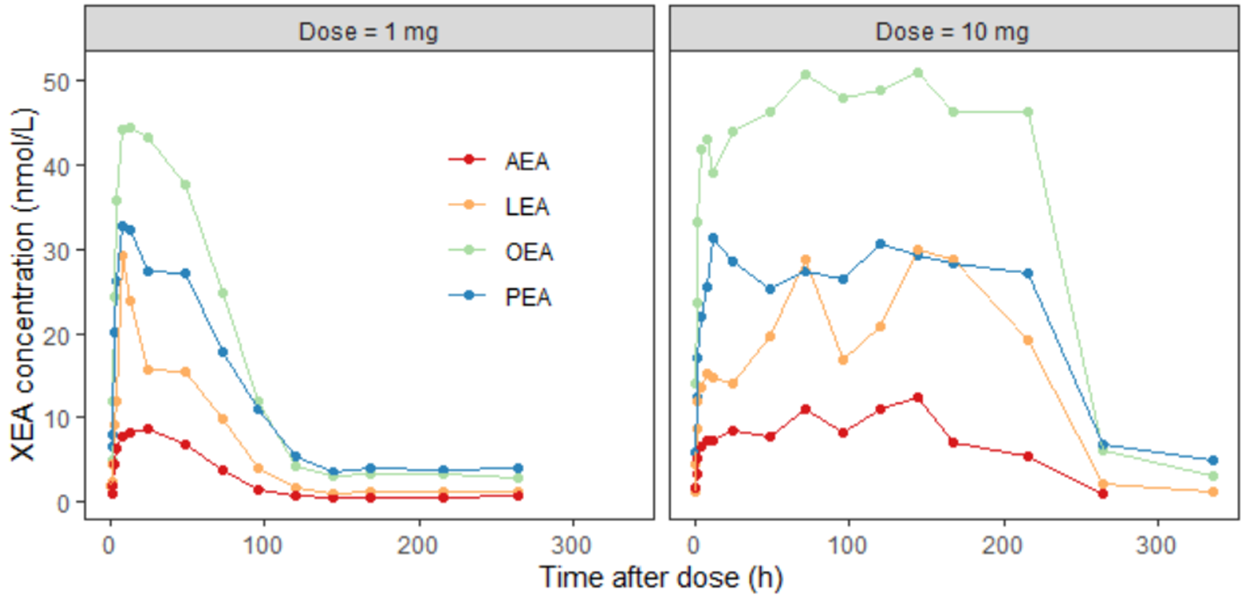
• the XEA concentration over time for two different dose levels

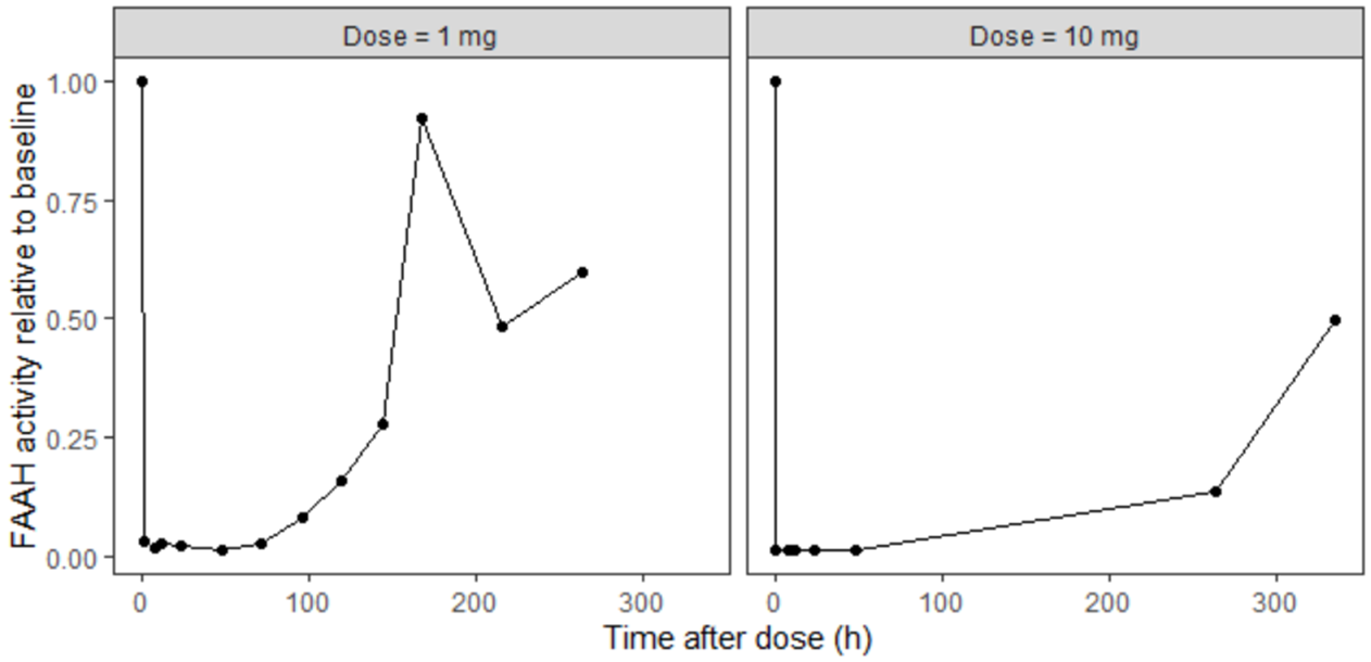
• and the FAAH activity relative to baseline for two different dose levels

Information from literature mostly came from in vitro experiments and data on rats, so it is limited but may give an idea about possible range of values.

• Fractions of each PX: BBRC (1996) vol 218. Rat testis

• Distribution of NAT across organs: J. Neuroscience, vol 17 (4). Rat

• Vmax and Km for PLD: JBC (2004) vol 279. In vitro experiments with mouse NAPE-PLD.

• Ki for PLD: Anal Biochem (2005) vol 339. In vitro experiments with mouse brain NAPE-PLD.

• Velocity FAAH: Biochemistry (1999) vol 38. In vitro experiment with rat brain FAAH.

• Distribution of FAAH across organs: BBA (1997) vol 1347. Rat.

• Km for FAAH: JBC (1995), vol 270 (11). In vitro experiments with rat brain FAAH.

• Distribution of NAAA across organs: JBC (2001) vol 276. Rat.

• Transport parameters: rapid equilibrium + internal logP measurements

• Organ volumes: J Pharmacokinet Pharmacodyn (2008) vol 35. Human.

• Kd for CB1: British Journal of Pharmacology (2007) vol 152. Human.

The parameter calibration process was split into two steps:

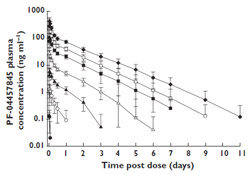
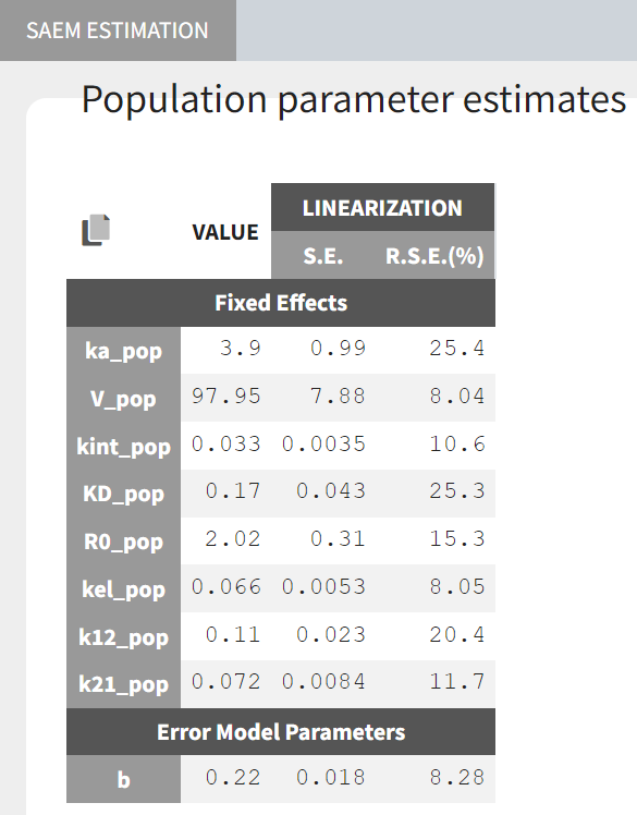
1. A PK model was developed and fitted to the averaged Phase I PK data, providing estimates for the 8 PK parameters.

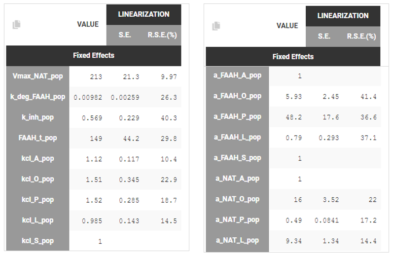
2. A PD model was then built. The PK parameters were fixed to the values from step 1, while 78 other parameters were fixed based on literature data. The remaining 10 parameters were estimated by fitting the model to the Phase I data.

PK Model

Development of the PK model is not the topic of this case study - see a step-by-step tutorial to learn about a typical PK workflow in Monolix - so the description contains only the final model.

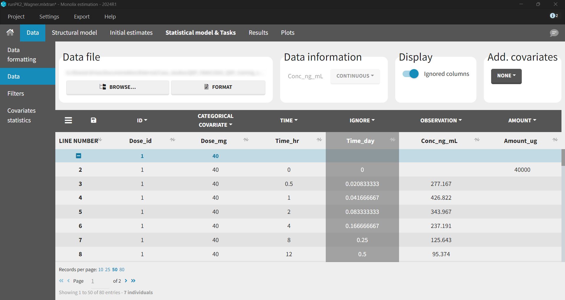
Because the PK data contained only the averaged information about concentration for several dose groups, the ID column indicates a dose group - not a typical individual subjects identifier. In addition, random effects were removed for all parameters.

Wagner TMDD model from the Monolix library accurately captured the averaged data as shown in the individual fits plot below - each subplot corresponds to a different dose group:

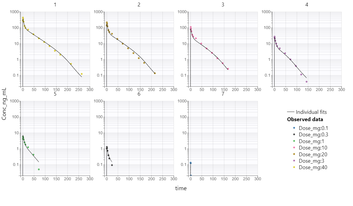
Estimated parameter values, together with the relative standard errors show good confidence in the estimated values.

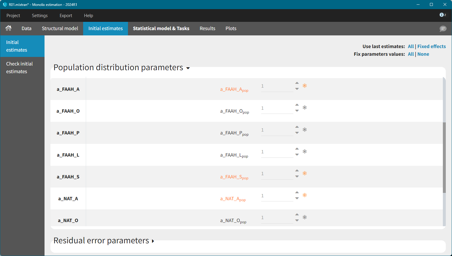
PD model

In the PD model:

• the PK parameters were fix in the model to values estimated in the previous step,

• 78 parameters were taken from the literature and were fixed directly in the structural model file,

• 10 parameters were estimated using the preclinical data on XEA concentration and FAAH activity.

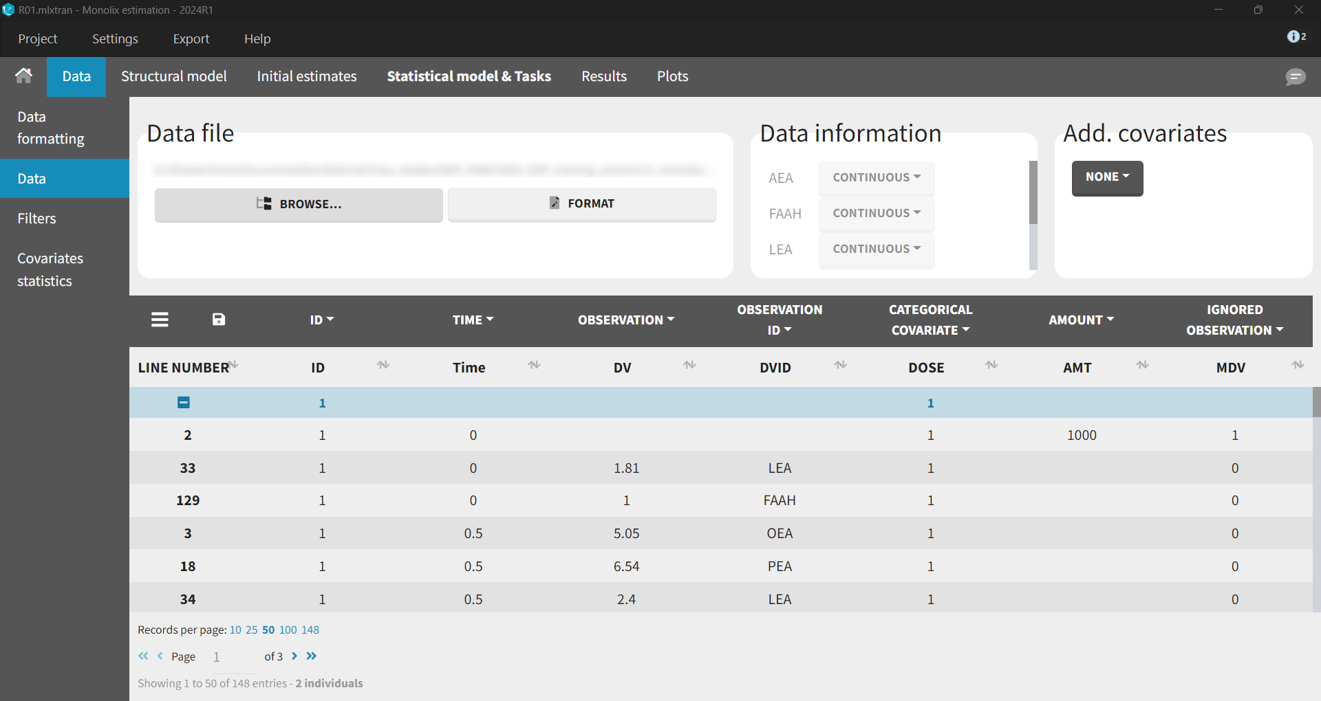
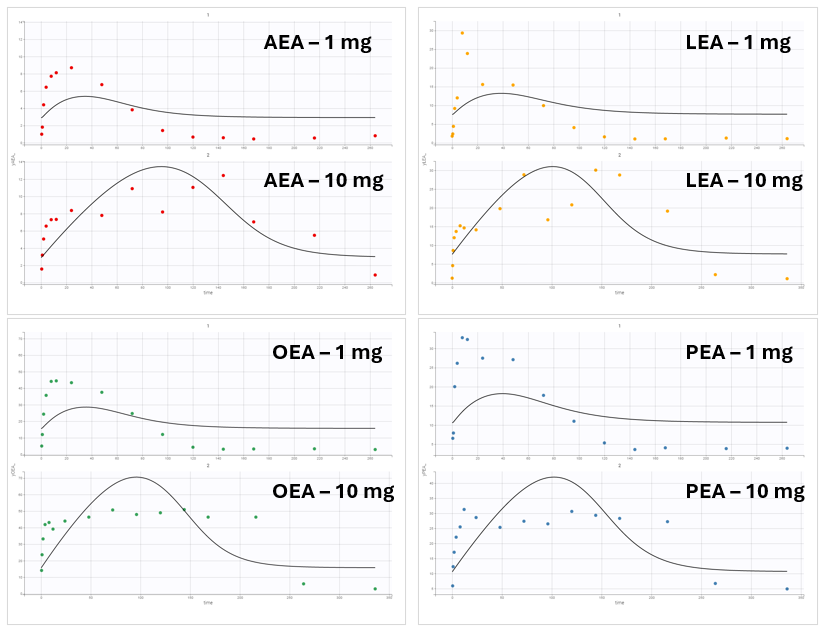
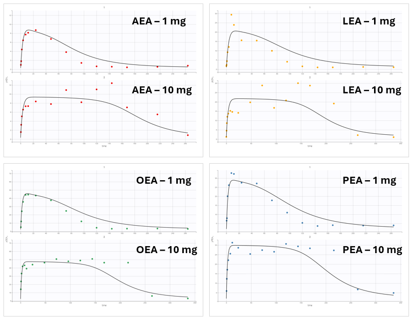
The data set contained XEA and FAAH measurements in the observation column, distinguished using identifiers (AEA, LEA, OEA, PEA, FAAH) in the observation ID column. The ID column, as previously, represented the two dose groups 1 mg (ID = 1) and 10 mg (ID = 2). In Monolix, these two groups are visulized in separate plots.

Base Model

After loading a model, Structural model tab displays the mapping between the observation-ID from the data set and the model outputs. This mapping can be adjusted using a drag-and-drop method.

Model exploration in Simulx gave the first insight on how parameters impact the predictions:

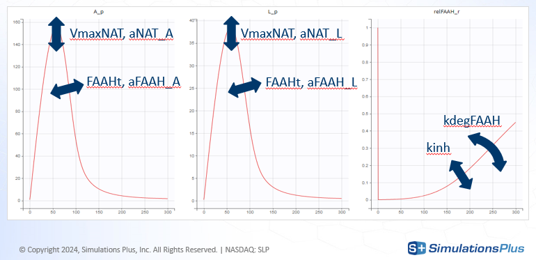
• kinh and kdegFAAH impact FAAH activity, which in turn impacts the XEAs

• VmaxNAT and FAAHt impact all XEAs

• aNAT_X and aFAAH_X allow to impact each XEA independently

  • aNAT_A = aFAAH_A = 1 as AEA is considered as a reference

  • aNAT_S = aFAAH_S = 1 because SEA is not observed

To identify suitable initial values for the remaining parameters, the Check initial estimates plot was used. The FAAH variable was inspected first.

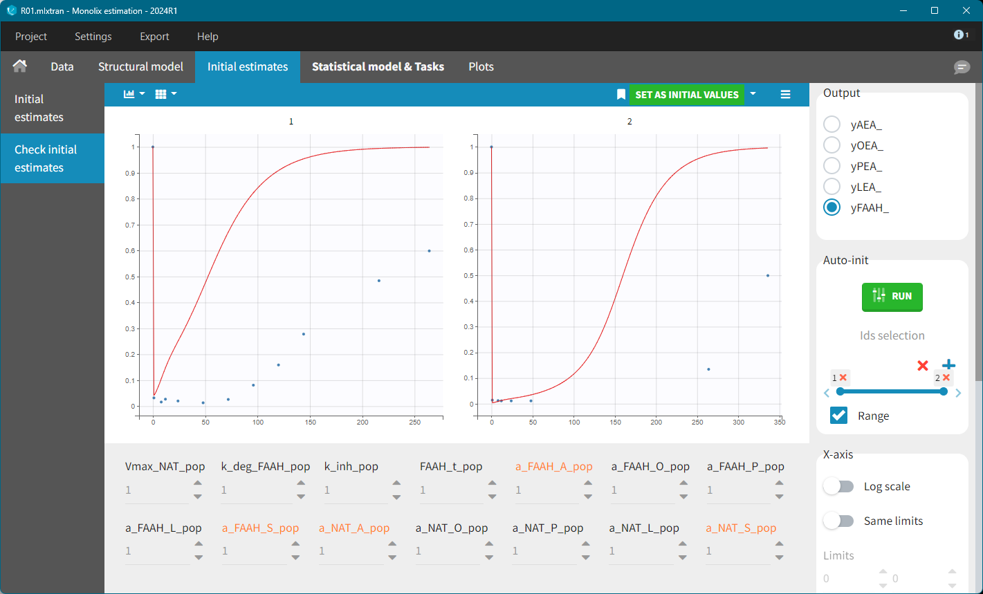
With default values, the predicted FAAH level increased back to their initial value too rapidly. The key parameters affecting this behavior are: k_deg_FAAH, kinh and FAAH_t. Setting k_deg_FAAH = 0.01 resulted in a better fit.

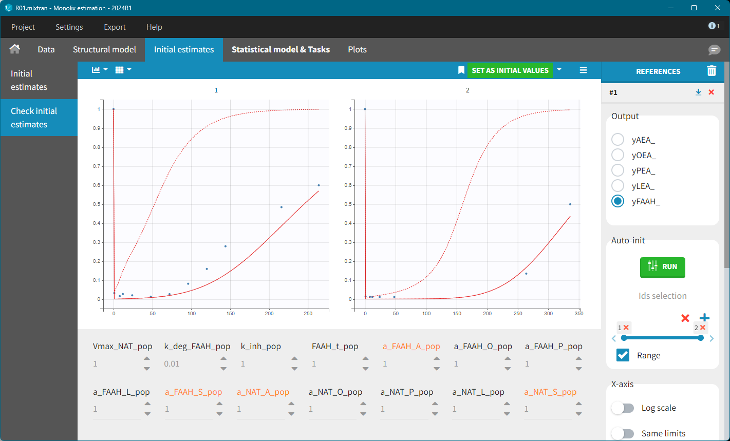
To refine the other initial parameter values, the AES plot was inspected, allowing for manual adjustments to reach a reasonable range. For example, the following values were tested:

Kdeg=0.01, Vmax=10, k_inh=0.1, FAAH=80, a_NAT_O=10, a_NAT_L = 10, a_NAT_P=0.5, a_FAAH_P=30.

Further refinement can be performed using the Auto-initialization feature.

This case study used only averaged data, without individual observations. As a result, inter-individual variability (i.e random effects) was removed from all parameters.

However, this model failed to accurately fit the clinical data as shown in the individual fits plot:

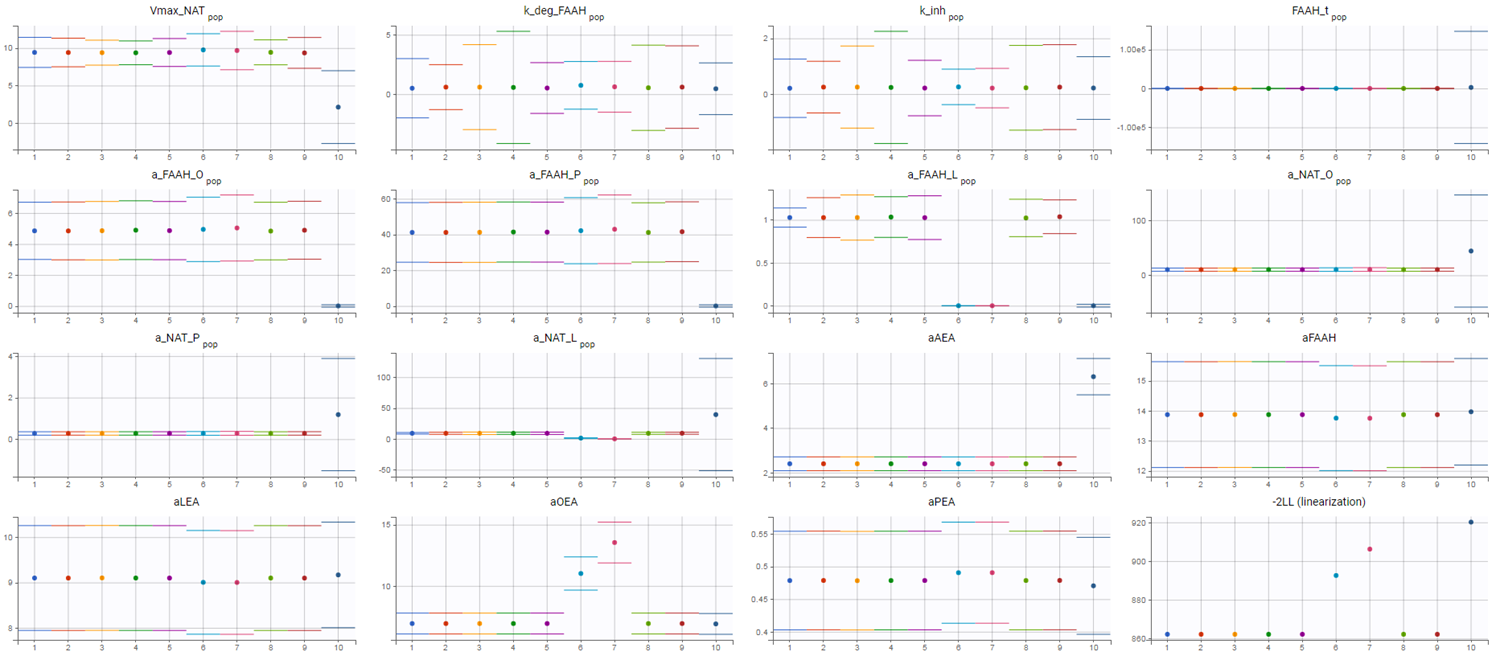
To investigate this issue, a convergence assessment was performed to evaluate sensitivity to initial values. The results showed that the algorithm consistently identified the same parameter estimates, except in three out of the ten runs. In those exceptions, the objective function value (as seen in the last plot showing the -2LL) was higher, indicating a poorer fit.
The convergence assessment shows that even starting from different intiial values, it is not possible to obtain a better fit than the one shown above.

Refining the Model: The Role of NAAA

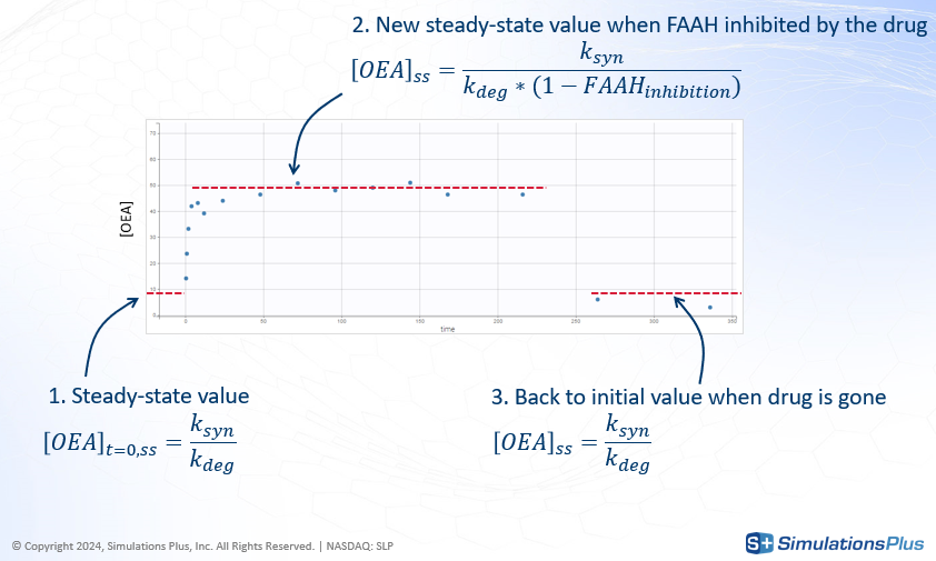
The discrepancy between model predictions and the observed data suggests that a key mechanism may be missing from the model. The XEA concentration data across all conditions exhibit a typical profile: an initial steady-state level, a sharp increase following drug administration, and a return to baseline as the drug is eliminated.

In the current model, XEA dynamics are governed by a production rate ksyn and a degradation rate kdeg, the latter depending on the concentration of FAAH. The steady-state concentration before dosing corresponds to the balance between these two rates.

1. Concentration profile starts from an initial value that represent the steady-state before the dose given by

2. Following drug administration, FAAH is inhibited, leading to a reduction in k_deg and, consequently, an increase in the steady-state concentration of XEA.

3. Once the drug is eliminated, FAAH activity recovers, and the XEA concentration returns to baseline.

To illustrate this, consider the FAAH data for the 10 mg dose group, where inhibition reaches approximately 97%.

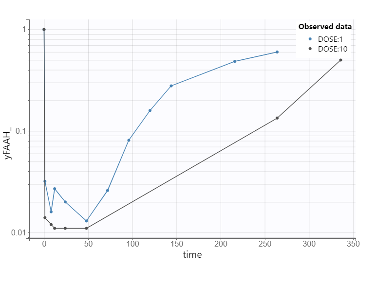
This level of inhibition should theoretically result in a 33-fold increase in the XEA steady-state concentration.

However, the experimental data show only a modest increase. So the fitting algorithm finds a compromise. The fitting algorithm slows down the rate of XEA accumulation, preventing it from reaching the new theoretical steady-state before the drug is cleared. This mismatch highlights a structural limitation of the model and suggests missing biology.

To better match the observed 5-fold increase in XEA concentrations, a secondary degradation pathway was considered. A new degradation term, kdeg2 = 0.21*kdeg was added to represent an FAAH-independent clearance mechanism.

Several enzymes are known to degrade XEAs. Based on literature evidence, NAAA (N-acylethanolamine acid amidase) was identified as a likely candidate. It has been shown to degrade multiple XEA species and exhibits Km values consistent with their physiological concentrations.

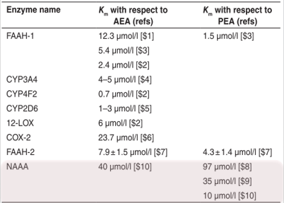
Incorporating NAAA-mediated degradation into the model significantly improved the fit. The model now correctly predicts the experimentally observed 5-fold increase in XEA levels upon FAAH inhibition. This refinement provided an important biological insight: AEAs are also degraded by NAAA, which limits the impact of FAAH inhibition. This mechanistic discovery emerged directly from the QSP modeling process.

Model Confidence and Uncertainty

To assess the reliability of the model and the robustness of the parameter estimates, two complementary methods were applied:

Fisher Information Matrix: Standard errors were computed using the Fisher Information Matrix. The results indicated that the estimated parameters had reasonably low uncertainty, suggesting good confidence in their values.

A second method in the Monolix GUI to asses population parameter uncertainty is bootstrap - based on sampling many replicate datasets and re-estimating parameters on each replicate. It is not shown in this case study.

Profile Likelihood: This complementary method was used to explore the parameter space and confirm that all estimated parameters were identifiable. For each parameter, its value is fixed incrementally above and below the estimated value, and the other parameters are re-estimated. The corresponding log-likelihood is recorded, generating a profile of the likelihood function.

To illustrate the principle, consider a simple two-parameter model with theta1 and theta2.

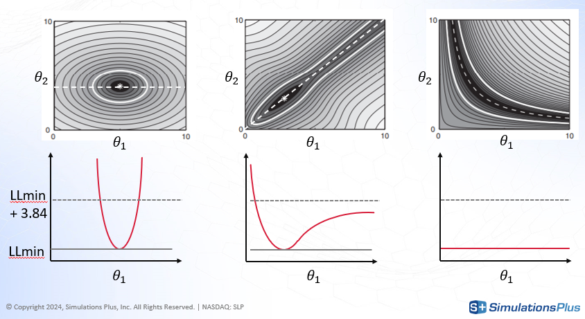
• The shaded gray region in the diagram (top) represents the likelihood landscape.

• The black area corresponds to the optimal parameter region.

• Fixing theta1 and re-estimating theta2 traces a path through the region of minimum likelihood (dashed line).

• The red curve (bottom) plots the log-likelihood (LL) along this path.

Case 1 (left): The log-likelihood increases sharply when theta1 deviates from its estimated value. This indicates a narrow confidence interval and high identifiability.

Case 2 (middle): The likelihood increases sharply when theta1 decreases, but only slowly when it increases. This asymmetry indicates partial identifiability — uncertainty exists in one direction.

Case 3 (right): The log-likelihood remains flat along the path, meaning that many combinations of theta1 and theta2 yield similar fits. This indicates non-identifiability.

Profile likelihood can be comupted using lixoftConnectors - see example.

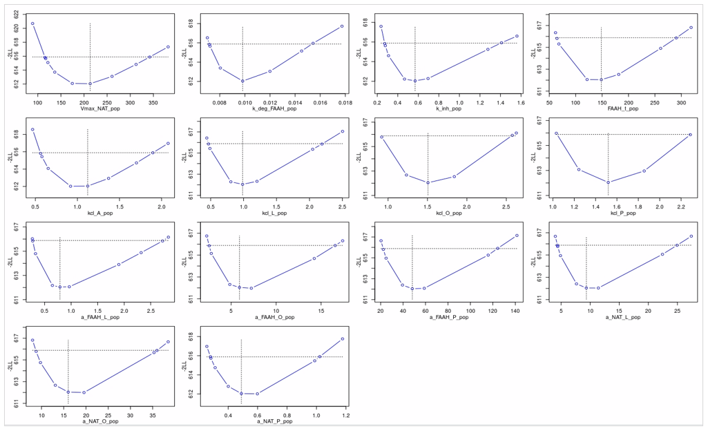
Applied to the PD model in this case study, profile likelihood analysis confirmed that all estimated parameters were practically identifiable. For each parameter, deviations from the estimated value resulted in a noticeable worsening of the model likelihood, reinforcing confidence in the parameter estimates.

Simulations

With the refined model and validated parameter estimates, simulations were performed to address the central question:

What dose is required to achieve a meaningful clinical effect?

Predicting CB1 Occupancy

The drug’s effect is mediated through the agonist action of AEA on CB1 receptors in the brain. CB1 occupancy depends on the brain concentration of AEA and its binding affinity, according to a standard receptor occupancy model.

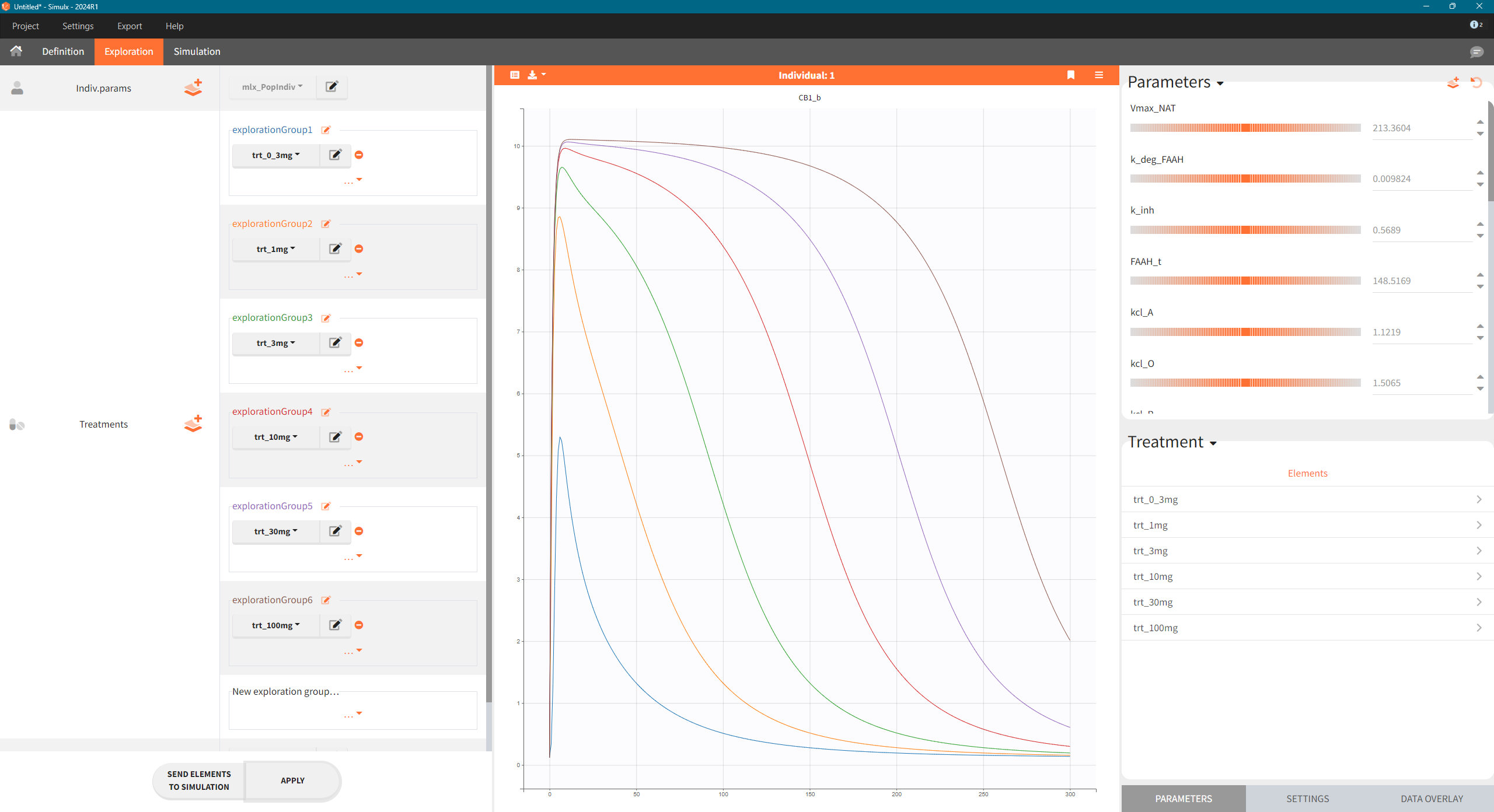
The model was used to simulate CB1 occupancy as a surrogate for drug effect. To explore the predicted CB1 occupancy at different dose levels, the final PD model was exported from Monolix to Simulx, and the following steps were performed:

• Export the final PD model R02_withNAAA.mlxtran from Monolix to Simulx,

• Define new treatment elements with different dose levels: type “manual” with a single dose of 0.3, 1, 3, 10, 30 and 100 mg at time t=0

• Define an output element with variable CB1_b of type “regular” from time 0 to 300 h

• Create scenario in the Exploration tab.

Simulations across various dose levels revealed that even at high doses, the CB1 occupancy plateaued at a low level (10%). This was a significant finding, suggesting that the drug, even with strong FAAH inhibition, may not be potent enough to achieve a therapeutic effect.

Sensitivity analysis

To understand the robustness of this prediction, a sensitivity analysis was performed. The goal was to identify which model parameters most strongly influence the predicted CB1 engagement.

The “absolute” sensitivity coefficient represents measures the change in CB1 occupancy resulting from a fixed change in a parameter’s value.

The “relative” sensitivity measures the percentage change in CB1 occupancy resulting from a proportional (e.g., 20%) change in the parameter value.

The relative sensitivity provides a normalized view of parameter influence, which is especially useful when parameters differ in scale or units.

The following R-script using lixoftConnectors calculates the percentage change in CB1 occupancy when each parameter is increased by 20%.

Step 1: Define and run reference simulation with default fixed parameters

initializeLixoftConnectors(software = "simulx")
# Path to model file
model <- 'model_3_allParam.txt'

# Create a new Simulx project
newProject(modelFile = model)

# Define parameter, treatment and output elements for simulation
defineIndividualElement(name = "param_ext", element = read.csv("param.csv", header = T))
defineTreatmentElement(name = "singleDose_10mg", element = list(data = data.frame(time = 0, amount = 10)))
defineOutputElement(name = "outCB1", element = list(data = data.frame(time = seq(0, 300, by = 1)), output = "CB1_b"))
defineOutputElement(name = "outAEA", element = list(data = data.frame(time = seq(0, 300, by = 1)), output = "A_p"))

# Run reference simulation
setGroupElement(group = "simulationGroup1", elements = c("param_ext", 
                                                         "singleDose_10mg",
                                                         "outCB1", "outAEA")
)
getGroups()
runSimulation()
ref <- getSimulationResults()
saveProject("ref_sim.smlx")

# Reference value for CB1 with default fixed parameters
CB1ref <- max(ref$res$CB1_b$CB1_b)

Step 2: Run a simulation for parameters values increased by 20% - loop over all parameters.

# Loop over all parameters
results <- data.frame()
resultsAll <- data.frame()
resultsAEA <- data.frame()

for(i in 1:ncol(df_params)){
  param_name <- names(df_params)[i]
  param_value <- df_params[[i]]*1.20
  df_temp_params <- df_params
  df_temp_params[i] <- param_value

  defineIndividualElement(name = "tempParam", element = df_temp_params)
  
  setGroupElement(group = "simulationGroup1", elements = c("tempParam", 
                                                           "singleDose_10mg",
                                                           "outCB1", "outAEA")
  )
  runSimulation()
  sim <- getSimulationResults()
  
  # calculate percent change from ref in CB1max
  CB1change <- abs(max(sim$res$CB1_b$CB1_b)-CB1ref)/CB1ref*100
  
  results <- rbind(results, data.frame(param = param_name, CB1change=CB1change))
  
  sim$res$CB1_b$param <- param_name
  sim$res$CB1_b$dir <- ifelse((max(sim$res$CB1_b$CB1_b)-CB1ref)/CB1ref>0, 1,0)
  sim$res$CB1_b$max <- CB1change
  resultsAll <- rbind(resultsAll, sim$res$CB1_b)
  
  sim$res$A_p$param <- param_name
  resultsAEA <- rbind(resultsAEA, sim$res$A_p)
}

results <- results %>% arrange(desc(CB1change))

Step 3: Re-organize data and plot the results

# Combining reference with simulation
refrep <- ref$res$CB1_b[rep(1:nrow(ref$res$CB1_b),times = length(df_params)),]
refrep$sim   <- 'ref'
refrep$param <- resultsAll$param
refrep$dir   <- resultsAll$dir
refrep$max   <- resultsAll$max
refrep$id    <- NULL

resultsAll$sim <- "changed"
resultsAll <- resultsAll[,c("time",'CB1_b','sim','param','dir','max')]

plotdf <- rbind(refrep,resultsAll)
plotdf$sim <- as.factor(plotdf$sim)
plotdf$param <- as.factor(plotdf$param)
plotdf <- plotdf[plotdf$param %in% results[1:9,"param"],] # select 9 param with most impact
plotdf <- plotdf %>% arrange(desc(dir),desc(max)) # sort 
plotdf$param <- factor(plotdf$param, levels = unique(plotdf$param)) # order factors for the plot

# Plotting
ggplot(plotdf)+geom_line(aes(x=time,y=CB1_b,color=sim),size=1)+
  ylab("CB1 occupancy")+
  xlab("Time (h)")+
  facet_wrap(~param)


# Rearranging AEA
refAEArep <- ref$res$A_p[rep(1:nrow(ref$res$A_p),times = length(df_params)),]
refAEArep$param <- resultsAEA$param
refAEArep$sim   <- 'ref'
resultsAEA$sim <- "changed"
resultsAEA <- rbind(resultsAEA,refAEArep)
resultsAEAb <- resultsAEA[resultsAEA$param=="b_NAT_Brain"|resultsAEA$param=="p_A"|resultsAEA$param=="b_NAAA_Brain",
                          c("time",'A_p','sim','param')]

ggplot(resultsAEAb)+geom_line(aes(x=time,y=A_p,color=sim),size=1)+
  ylab("AEA concentration (nM)")+
  xlab("Time (h)")+
  facet_wrap(~param)

resultsCB1b <- plotdf[plotdf$param=="b_NAT_Brain"|plotdf$param=="p_A"|plotdf$param=="b_NAAA_Brain",]
resultsCB1b$param <- factor(resultsCB1b$param, levels = c("b_NAAA_Brain","b_NAT_Brain","p_A"))
ggplot(resultsCB1b)+geom_line(aes(x=time,y=CB1_b,color=sim),size=1)+
  ylab("CB1 occupancy")+
  xlab("Time (h)")+
  facet_wrap(~param)

Parameters having the largest relative sensitivity:

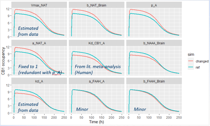
For the two last parameters, the impact is minor - it means that the impact is minor also for all other parameters.

• The parameter a_NAT_A is fixed to 1 in the model, serving as a reference value for the other XEA species.

• The binding affinity of AEA, Kd_CB1_A, is based on human experimental data, and is therefore considered reliable.

• Parameters Vmax_NAT and kcl_A were estimated directly from the available data, and their confidence intervals indicate a high degree of certainty in their values.

The three remaining parameters showed a potentially meaningful impact on CB1 predictions and warranted closer examination. Their influence was analyzed by plotting the effect on CB1 occupancy (top panel), and the effect on observed AEA concentrations (bottom panel).

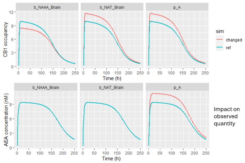
• Parameter p_A impacts the AEA concentration. Probably during parameter estimation, changes in p_A could be compensated by adjustments in other unfixed parameters, leading to the same CB1 outcome. This kind of compensation can lead to a situation where prediction remains stable even if certain parameters are not precisely known.

• In contrast, the two remaining parameters (b_NAAA_Brain and n_NAT_Brain) had no observable effect on the AEA data, yet had a substantial influence on CB1 occupancy predictions. These parameters were not estimated, but fixed based on rat-derived literature values, which introduces uncertainty.

Because these parameters strongly affect CB1 predictions while remaining unconstrained by the observed data, the model’s prediction of CB1 occupancy in humans remains uncertain. This highlights the importance of:

• Using species-relevant data for key translational parameters, and

• Performing sensitivity analysis to identify where uncertainty in inputs may critically impact conclusions.

Conclusions

This case study shows the critical value of QSP modeling in drug development.

• First, despite the uncertainty of the parameters, the modeling uncovered a key biological mechanism—the role of the NAAA enzyme—that was not initially considered. This finding can have significant implications - a combination therapy targeting both FAAH and NAAA might be a more effective strategy.

• Second, the model provided a dose-response prediction, showing that even with high doses, the FAAH inhibitor may not be able to achieve a clinically meaningful CB1 occupancy.

• Finally, the sensitivity analysis revealed that this prediction was highly sensitive to parameters. –Even if CB1 occupancy would be known, its effect on pain remain unknown. This highlighted a significant uncertainty of the pharmacological effect in Phase II and provided guidance for future research—either to gather more data to better characterize these parameters or to re-evaluate the project's viability.

Ultimately, this QSP model served not just as a tool for fitting data, but as a framework for integrating knowledge, identifying gaps, and informing strategic decisions in a complex drug development project.