
Download data set only | Download all Monolix & Simulx project files V2021R2 | Download all Monolix & Simulx project files V2023R1 | Download all Monolix & Simulx project files V2024R1
This case study demonstrates how to implement and analyze a longitudinal MBMA model using Monolix and Simulx. See also the published tutorial in CPT: PSP.
Introduction
Model-based meta-analysis (MBMA) is a quantitative approach that can integrate previously published aggregate data (for example, mean responses over treatment arms) from multiple studies with other, possibly unpublished, data to inform key drug development decisions. For example, MBMA can be used to decide if a treatment under investigation has a reasonable chance of showing clinical benefit compared to existing treatments.
The importance of MBMA for internal decision-making is well recognized, however, its role and contribution within model-informed drug development is not yet well established (Chan P et al).
Key applications of MBMA include:
-
Leveraging prior knowledge from multiple sources for strategic decision-making
-
External benchmarking and competitor selection
-
Informing the target product profile, proof of concept to Phase 3 dose selection and study design, as well as quantifying probability of trial success (Naik H et al)
-
Comparing multiple treatment options, not tested in head-to-head trials
Informing disease progression models
Data used for an MBMA analysis consist of summary study-level data (for example, pain score averaged over the trial arm) extracted from published literature. Individual data are usually not available as only average responses over entire treatment arms are reported in publications. The data are typically longitudinal (over time), though MBMA for landmark data (a single time point) has been described too. Data collection should ideally follow Preferred Reporting Items for Systematic reviews and Meta-Analyses (PRISMA) guidelines, and assessing a lack of publication bias is recommended.
Glossary
|
ACR20 |
20% improvement in the American College of Rheumatology response criteria |
|
AIC |
Akaike information criterion |
|
BIC |
Bayesian information criterion |
|
BSV |
between-study variability |
|
BTAV |
between-treatment-arm variability |
|
CV |
coefficient of variation (expressed as a percent) |
|
Emax |
maximal response to the drug |
|
EmaxFE |
fixed effect of maximal response to the drug |
|
etaBSVEmax |
between-study variability maximal response to the drug |
|
etaBTAVEmax |
between-treatment-arm variability maximal response to the drug |
|
IIV |
interindividual variability |
|
IOV |
interoccasion variability |
|
MBMA |
model-based meta-analysis |
|
MTX |
methotrexate |
|
NaN |
not a number |
|
Narm |
number of individuals per arm |
|
Nik |
number of individuals in treatment group k of study i |
|
PRISMA |
Preferred Reporting Items for Systematic reviews and Meta-Analyses |
|
RA |
rheumatoid arthritis |
|
SAEM |
stochastic approximation expectation maximization |
|
SD |
standard deviation |
|
t |
time |
|
T50 |
time to achieve 50% of the maximum response |
Theoretical Concepts Underlying an MBMA
As an extension of traditional meta-analysis methodology, MBMA allows the incorporation of additional aggregate trial data information such as dose-response and longitudinal data (repeated measures) by way of parametric models. Similar to traditional meta-analyses, the underlying statistical models can include either only fixed effects or fixed and random effects. As illustrated in Figure 1, the main difference between fixed effects and fixed plus random effects MBMA is the lack or presence, respectively, of between-study variability (BSV) in treatment effect according to the definition in Boucher M and Bennetts M (2018).
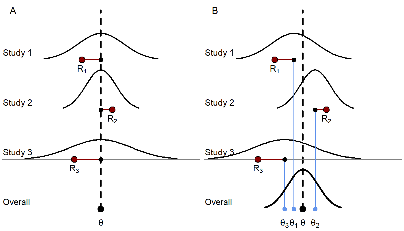
Figure 1. A) A fixed-effects model where each red dot represents a study result estimating a response, R. The underlying true effect, θ, is assumed to be identical across studies, that is, as no BSV in treatment effect is included (other than that due to covariates), thus, the deviation for each study from the true effect is assumed to be due to random sampling error. The sampling error is due to the sample not being perfectly representative of true population. A study with a smaller sample size would be more likely to produce an estimate farther from the true effect and would have a wider distribution. The differences in observed study effects are modeled as resulting from covariate effects and random sampling error. B) A random effects model where each study is assumed to have its own true trial-specific effect, θi, which comes from a distribution with mean θ and is observed with random sampling error as Ri. The differences in observed study effects are modeled as resulting from covariate effects, random sampling error (which, again, can depend on the sample size of each study), and additional BSV, which can be generalized to include between-treatment-arm variability (BTAV) as well.
Random effects MBMA models of study-level data may include components describing BSV, BTAV, and residual error (Ahn JE and French JL). This is similar to an analysis of individual-level data using nonlinear mixed-effects models, where this corresponds to the general approach of including interindividual variability (IIV), interoccasion variability (IOV), and residual error components (Table 1). Also, similar to the analysis of individual-level data, an MBMA may assess the impact of covariates on BSV and BTAV (“meta-regression” in traditional meta-analysis terms or “covariate analysis” in nonlinear mixed-effects modeling terms).
|
Table 1. Variability in an MBMA Mapped to Variability in a Population Analysis |
|
|
MBMA |
Population Analysis |
|
Between-study variability |
Interindividual variability |
|
Between-treatment arm variability |
Interoccasion variability |
|
Residual error or unexplained variability |
Residual error or unexplained variability |
In line with the traditional meta-analysis framework for analysis of aggregate trial data, MBMA accounts for the relative contribution of studies based on either: i) precision of the effect, that is, weighting via the empirical standard error or standard deviation (SD) of the reported mean effect(s) or ii) sample size, assuming equal precision within each included study and across time points (Boucher M and Bennetts M (2018)). In an MBMA, weighting is performed on the residual error and, if estimated, the BTAV component (Ahn JE and French JL). This weighting comes from starting with a linear individual-level model of response across studies with random effects for study and individual. Then a study-level model can be derived by taking the mean response per treatment group at specific time points of the individual-level model, where the mean depends on the number of individuals in treatment group k of study i, Nik. Thus, the study-level model has random effects for study as well as the mean per treatment group of the combined random effects for individuals and the random error, which can be replaced with a random arm effect and residual error which would both be weighted by √Nik. When relaxing the linear model assumption to consider nonlinear random effects, closed solutions are no longer possible, but approximations retain the same partitioning of BSV, BTAV, and a residual error term. See Ahn JE and French JL for a complete derivation. Note that weighting the residual error by the empirical standard error is preferred over weighting by sample size if that information is available over time, as this avoids the assumption that this variability is the same across studies and times (Boucher M and Bennetts M (2018)).
How do we interpret that BSV is not weighted while BTAV and residual error are weighted? Between-study variability represents the factors that differ among studies, such as design, inclusion criteria, location, and equipment, which are independent of the number of individuals recruited. Therefore, increasing the number of individuals in each study will not affect the BSV. However, BTAV is due to the characteristics of treatment arms not being identical following randomization since there is a finite number of individuals in each arm. The larger the number of individuals in each arm, the smaller the expected difference is between the mean characteristics of the arms, since one averages over a larger number. This is why the BTAV component in an MBMA is weighted by √Nik (or the precision, which incorporates the sample size). For the residual error, the reasoning is the same: as the individual-level residual error is averaged over a larger number of individuals, the study-level residual error decreases.
MBMA in Rheumatoid Arthritis
One benefit of an MBMA approach is determining, early on in development, if the new drug candidate has a reasonable chance of showing clinical benefit, over other comparator compounds.
Because an MBMA approach considers studies instead of individuals, the formulation of the problem as a mixed-effects model differs slightly from the typical model formulation in pharmacokinetic/pharmacodynamic analyses. This case study highlights how MBMA models can be implemented, analyzed, and used for decision support in Monolix and Simulx.
In the following case study, we focus on longitudinal data for the clinical efficacy of drugs for rheumatoid arthritis (RA). The goal is to evaluate the efficacy of a drug in development (Phase 2) in comparison to 2 drugs already on the market. This case study is inspired by Demin I et al.
Canakinumab, a Drug Candidate for Rheumatoid Arthritis
Rheumatoid arthritis is a complex autoimmune disease, characterized by swollen and painful joints. It affects around 1% of the population and evolves slowly (the symptoms manifest over months). Patients are usually first treated with traditional disease‑modifying anti-rheumatic drugs, the most common being methotrexate (MTX). If the improvement is too limited, patients can be treated with biologic drugs in addition to the MTX treatment. Although biologic drugs have an improved efficacy, remission is not complete in all patients. To address this unmet clinical need, a new drug candidate, canakinumab, has been developed at Novartis. After a successful proof-of-concept study, a 12-week, multicenter, randomized, double-blind, placebo-controlled, parallel‑group, dose-finding Phase 2B study with canakinumab + MTX was conducted in patients with active RA despite stable treatment with MTX. In the study, canakinumab + MTX was shown to be superior to MTX alone.
This case study compares the expected efficacy of canakinumab with the efficacy of 2 other biologics already on the market, adalimumab and abatacept. Several studies involving adalimumab and abatacept have been published. Those chosen to inform our case study are included in Table 2 below). A typical endpoint in the selected studies was a 20% improvement in the American College of Rheumatology response criteria (ACR20) (Felson DT et al), that is, the percent of patients achieving 20% improvement. In this case study, the particular focus in on longitudinal ACR20 data, measured at several time points after initiation of treatment, and a mixed‑effect model is used to describe these data.
Data selection, extraction, and visualization
Data selection
To compare canakinumab to adalimumab and abatacept, we searched for published studies involving these drugs. Reusing the literature search presented in Demin I et al, we selected only the studies with inclusion criteria similar to the canakinumab study, in particular: approved dosing regimens and patients having an inadequate response to MTX. In addition to the studies culled from Demin I et al, we included two additional studies published later (also included in Table 2). In all selected studies, the compared treatments were MTX + placebo and MTX + biologic drug.
|
Table 2. Full List of Publications Identified for the Case Study |
|||
|
Reference Link |
Manuscript Title |
Clinical Phase / Study Duration |
Treatment Arms/ Number of Patients / Dosing Regimens |
|
Subcutaneous abatacept versus intravenous abatacept: A phase IIIb noninferiority study in patients with an inadequate response to methotrexate |
Phase IIIb
|
SC abatacept 125 mg QW after an IV LD (~10 mg/kg) (n = 736) IV abatacept (~10 mg/kg) on Days 1, 15, 29 and Q4W (n = 721) |
|
|
Radiographic, clinical, and functional outcomes of treatment with adalimumab (a human anti-tumor necrosis factor monoclonal antibody) in patients with active rheumatoid arthritis receiving concomitant methotrexate therapy: a randomized, placebo-controlled, 52-week trial |
Phase III
|
SC adalimumab 40 mg Q2W (n =207) SC adalimumab 20 mg Q2W (n =212) Placebo Q2W (n=200) |
|
|
A randomized, double-blind, placebo‑controlled, phase III study of the human anti-tumor necrosis factor antibody adalimumab administered as subcutaneous injections in Korean rheumatoid arthritis patients treated with methotrexate |
Phase III 6 months |
SC adalimumab 40 mg Q2W (n =65) Placebo (n=63) |
|
|
Treatment of rheumatoid arthritis with the selective costimulation modulator abatacept: Twelve-month results of a phase IIb, double-blind, randomized, placebo-controlled trial |
Phase IIb 12 months |
abatacept 10 mg/kg (n = 115) abatacept 2 mg/kg (n = 105) Placebo (n=119) All TRT on Days 1, 15, 29 and Q4W |
|
|
Effects of abatacept in patients with methotrexate-resistant active rheumatoid arthritis: a randomized trial |
Phase III 12 months |
abatacept ~10 mg/kg (n = 433) Placebo (n=219) All TRT dosed Q4W |
|
|
Efficacy and safety of abatacept or infliximab vs placebo in ATTEST: a phase III, multi-centre, randomised, double-blind, placebo-controlled study in patients with rheumatoid arthritis and an inadequate response to methotrexate |
Phase III 12 months |
abatacept 10 mg/kg Q4W (n = 156) Infliximab 3 mg/kg Q8W (n = 165) Placebo (n=110) |
|
|
Adalimumab, a fully human anti-tumor necrosis factor alpha monoclonal antibody, for the treatment of rheumatoid arthritis in patients taking concomitant methotrexate: the ARMADA trial |
Phase III
|
SC adalimumab 20 mg Q2W (n =69) SC adalimumab 40 mg Q2W (n =67) SC adalimumab 80 mg Q2W (n =73) Placebo Q2W (n=62) |
|
|
Head-to-head comparison of subcutaneous abatacept versus adalimumab for rheumatoid arthritis: findings of a phase IIIb, multinational, prospective, randomized study |
Phase IIIb
|
SC abatacept 125 mg QW (n = 318)
|
|
|
Abbreviations: IV, intravenous; LD, loading dose; n, numbers of patients; Q2W, every 2 weeks; Q4W, every 4 weeks; Q8W, every 8 weeks; QW, every week; SC, subcutaneous; TRT, treatment. |
|||
Data extraction
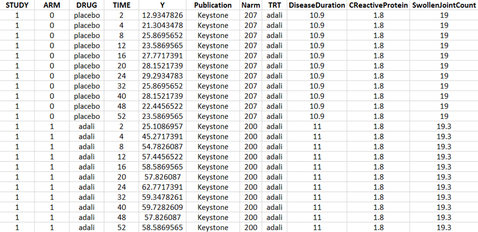
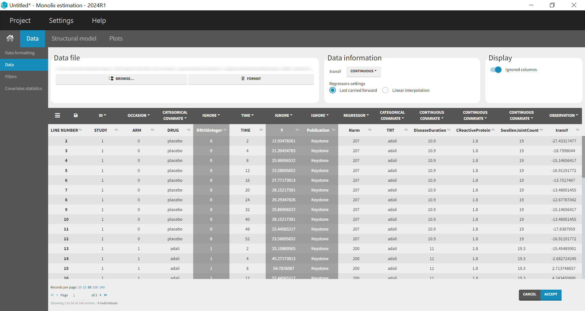
Using a data digitizer, we extracted the longitudinal ACR20 data from the selected publications listed in Table 2. The information was recorded in a data file, together with additional information about the studies. The in-house individual canakinumab data from the Phase 2 trial was averaged over the treatment arms to be comparable to the literature aggregate data. Below is a screenshot of an excerpt of the data file and a description of the columns.
-
STUDY: index of the study/publication (equivalent to the ID column)
-
ARM: 0 for placebo arm (that is, MTX + placebo treatment), and 1 for biologic drug arm (MTX + biologic drug)
-
DRUG: name of the drug administrated in the arm (placebo, adalimumab, abatacept, or canakinumab)
-
TIME: time since beginning of the treatment, in weeks
-
Y: ACR20, percentage of persons on the study having an at least 20% improvement of their symptoms
-
Publication: first author of the publication from which the data has been extracted
-
Narm: number of individuals in the arm
-
TRT: treatment studied in the study
-
DiseaseDuration: mean disease duration (in years) in the arm at the beginning of the study
-
CReactiveProtein: mean C-reactive protein level (in mg/dL)
-
SwollenJointCount: mean number of swollen joints
Data visualization
Monolix contains an integrated data visualization module, which is very useful to gain an overview and understanding of the data after importing it. After creating a new project in Monolix, we clicked on Browse in the Data file option to select the data file. The dataset columns are assigned in the following way:
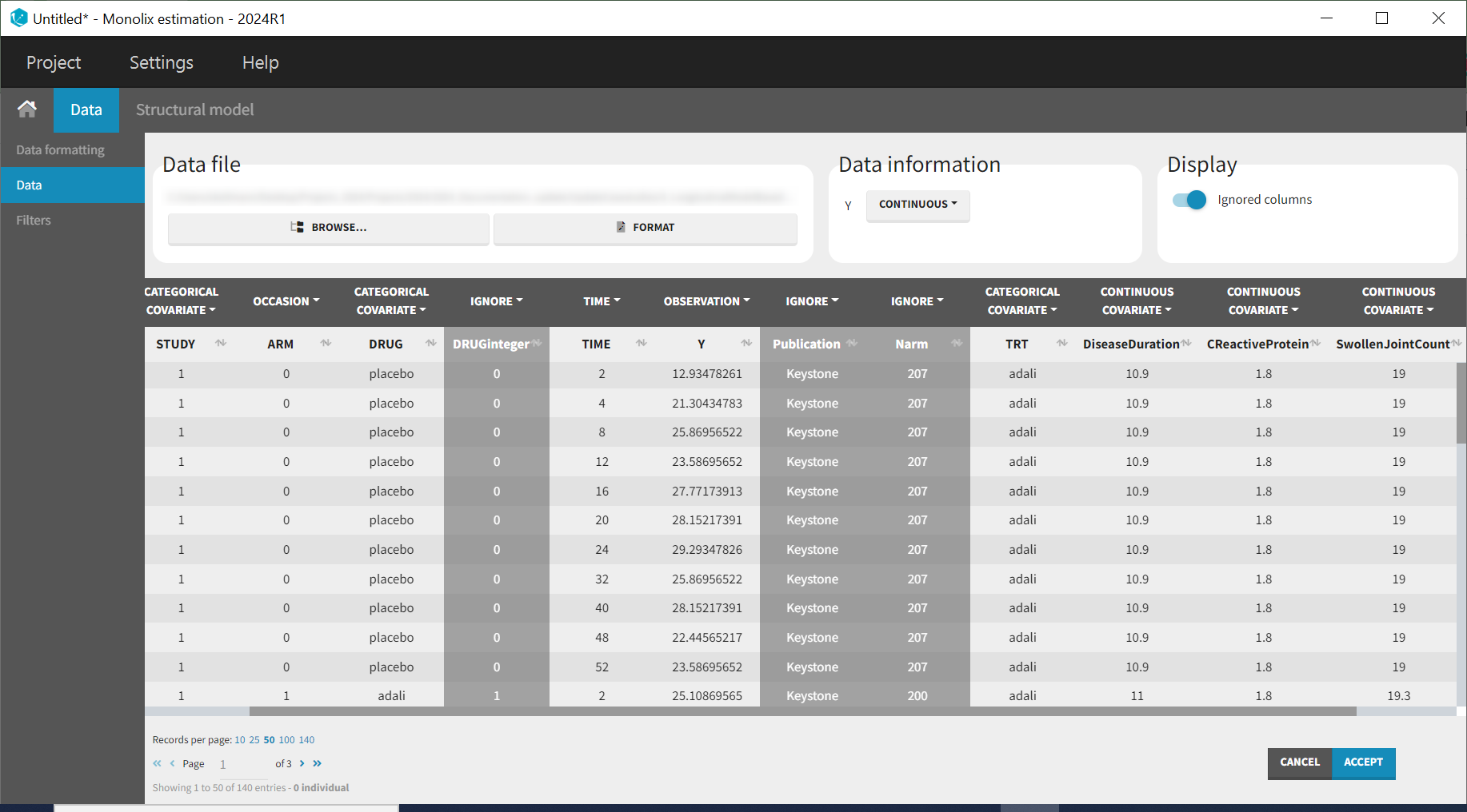
The STUDY column is tagged as ID, and the ARM column is tagged as OCCASION, as the IIV and IOV concepts in MonolixSuite are used to define BSV and BTAV. All columns that may be used to stratify/color the plots must be tagged as either continuous or categorical covariates, even if these columns will not be used in the model.
After clicking ACCEPT and NEXT, the data appear in the Plots tab. To better distinguish the treatments and arms, the STRATIFY tab will allow us to allocate the DRUG and TRT covariates. Then choose to split by TRT and color by DRUG. Also arrange the layout in a single line. In the X-AXIS section of the SETTINGS tab, apply the toggle for custom limits, which automatically sets the limits to 1 and 52.14. In the figure below, arms with biologic drug treatment appear in color (abatacept in blue, adalimumab in red, canakinumab in green; customized color selection), while placebo arms appear in black. Note that even in the “placebo” arms, the ACR20 improves over time, due to the MTX treatment. In addition, we clearly see that the treatment MTX + biologic drug has better efficacy compared to MTX + placebo. For canakinumab, which is the in-house drug in development, only 1 study is available, the Phase 2 trial.
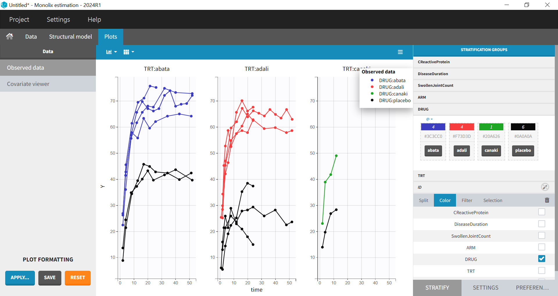
Given these data, we would like to know whether canakinumab has a chance to be more efficacious than adalimumab and abatacept. A longitudinal mixed-effect model was developed to address this.
Longitudinal mixed-effect model description
The ACR20 is a clinical threshold (Gaujoux-Viala C et al) and a patient who achieves this threshold is considered a responder. Given the time-course of the percent of patients achieving ACR20 criteria, the observed data to be a continuous variable bounded by 0, 100 is assumed, so an Emax structural model is proposed, which can be described by an Emax function as follows:
Where f(t) represents the percent of patients achieving ACR20 over time, Emax describes the maximal response to the drug, t is the time (weeks), and T50 is the time to reach half of the maximal response (weeks). While we want to estimate IIV and residual error, we need to ensure that the predictions remain bounded in the 0, 100 interval. In order to enable this, the aforementioned Emax equation is logit transformed.
A link function, such as the logit function, maps this bounded distribution to real numbers (
). Thus, if the individual parameter,
, is bounded between zero and 1, its logit is normally distributed.
The inverse transformation yields the original bounded parameter.
The logit transformation enables estimation of residual error that is normally distributed for the logit transformed model prediction f(t).
The percent of responders in the ith study, at the jth time point, and the kth treatment arm, with residual error 𝜖𝑖𝑗𝑘 is given by
Emaxik and T50ik are then the respective maximal response to the drug and the time to reach half of the maximal response for the ith study and the kth treatment arm.
The residual error,
, is distributed according to the following equation:
Where Nik is the number of individuals in treatment arm k of study i. Note the residual error is weighted by Nik. Since our data are scarce and our interest is estimation of the treatment-specific Emax (efficacy), we estimate BSV and BTAV for Emax only. The Emax cannot exceed 100, hence, in order to estimate the aforesaid variability, we logit transform it as follows, hereby transforming the Emax to the continuous parameter space.
with
represents the BSV and
represents the BTAV.
For T50, we select a log-normal distribution and no random effects:
with Emaxpopd and T50popd representing the typical population parameters,that depend on the administrated drug d. The BSV (index (0)) and BTAV (index (1)) terms for Emax have the following distributions:
Note that the BTAV and residual error are weighted by the number of individuals per arm, while the BSV is not, as explained in Theoretical Concepts Underlying an MBMA.
In the next section, we describe how to implement this model in Monolix.
Set Up of the Model in Monolix
Error Model Specification
We start by transforming both the ACR20 observations in the dataset and the model predictions in the following way so that the predefined constant error model may be implemented. Thus, we can rewrite:
where
is a constant unweighted residual error term. Next we multiply both sides by
to get rid of the denominator for
.
Finally, we can define
as the transformation applied to both the data and the model prediction in the equation:
Therefore, we have
-
, the transformed data (note, the observations need to be in the range zero to 1),
-
the transformed model prediction.
This data transformation is added to the dataset, in the column transY.
At this stage, we can load the new dataset with the transY column into Monolix and assign the columns as before, except that we now use the column transY as OBSERVATION.
STUDY is tagged as ID, ARM as OCCASION, DRUG as CATEGORICAL COVARIATE, TIME as TIME, transY as OBSERVATION, Narm as REGRESSOR, TRT as CATEGORICAL COVARIATE and DiseaseDuration, CReactiveProtein and SwollenJointCount as CONTINUOUS COVARIATE.
To match the observation transformation in the dataset, the Mlxtran model file will include the following:
ACR20 = ...
pred = logit(ACR20)*sqrt(Narm)
OUTPUT:
output = pred
In order to be available in the model, the dataset column Narm must be tagged as regressor, and passed as argument in the input list:
[LONGITUDINAL]
input = {..., Narm}
Narm = {use=regressor}
In our example, the number of individuals per arm (Narm) is constant over time. In cases of dropouts or non-uniform trials, Narm may vary over time. This will be taken into account in Monolix, as regressors can change over time.
Parameter Distribution
Similarly to the error model, it is not possible to weight the BTAV directly via the Monolix GUI. As an alternative, we can define separately the fixed effect (EmaxFE), BSV random effects (etaBSVEmax), and BTAV random effects (etaBTAVEmax) in the GUI and reconstruct the parameter value within the model file. Because we have defined Narm as a regressor, we can use it to weight the BTAV terms. We also need to be careful about adding the random effects on the normally distributed transformed parameters. Here is the syntax for the structural model:
[LONGITUDINAL]
input = {EmaxFE, T50, etaBSVEmax, etaBTAVEmax, Narm}
Narm = {use=regressor}

EQUATION:
; transform the Emax fixed effect (EmaxFE) to tEmax (normally distributed)
tEmax = logit(EmaxFE)

; adding the random effects (RE) due to between-study variability and
; between arm variability, on the transformed parameters
tEmaxRE = tEmax + etaBSVEmax + etaBTAVEmax/sqrt(Narm)

; transforming back to have EmaxRE with logit distribution (values between 0 and 1)
Emax = exp(tEmaxRE)/(1+exp(tEmaxRE))

; defining the effect
ACR20 = Emax * (t / (T50 + t))

; adding a saturation to avoid taking logit(0) (undefined) when t=0
ACR20sat = min(max(ACR20,0.01),0.99)

; transforming the effect ACR20 in the same way as the data
pred = logit(ACR20sat)*sqrt(Narm)

OUTPUT:
output = pred
In addition to the steps already explained, we add a saturation ACR20sat = min(max(ACR20, 0.01), 0.99) to avoid having ACR20=0 when t=0, which would result in pred = logit(0)(which is undefined).
In the structural model tab, we click on 'New model,' copy-paste the code above, and save the model. The model appears below.
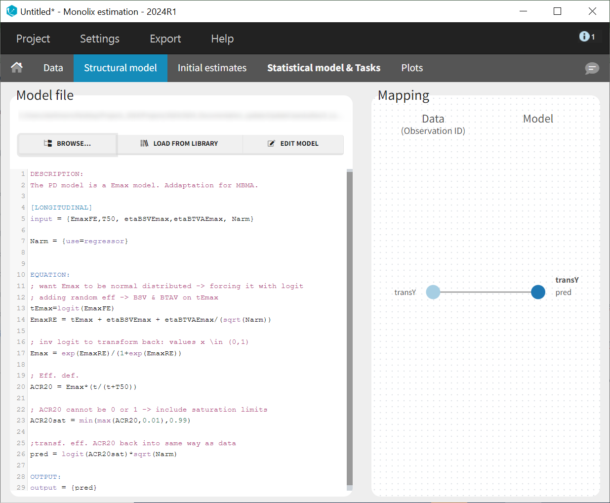
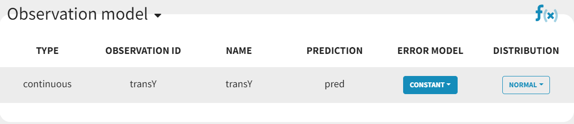
In the next tab, Statistical Model & Tasks, , we define the statistical part of the model. For the observation model, we choose constant from the list, based on the data transformation we performed above.
For the parameter distributions, we choose a logit-normal distribution for EmaxFE with distribution limits between zero and 1 (note that the default initial value for EmaxFE is 1 leading to default logit limits (0, 2), so the initial estimate for EmaxFE needs to be changed first, before its distribution can be set to logit-normal (bounded within (0, 1)) in the GUI. For time to achieve 50% of the maximum response (T50), a log-normal distribution is selected, while, for the random effects etaBSVEmax and etaBTAVEmax, a normal distribution is selected. The parameter EmaxFE assumes a normal distribution in the logit space, hence, can take values from
to
.
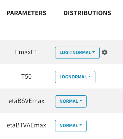
With this parametrization, EmaxFE represents only the fixed effects, so we need to disable (unselect) the random effects for this parameter, as well as for T50. etaBTAVEmax is the IOV, thus, we disable the RE at the STUDY level (shown as “ID” in the GUI) but enable them at the ARM level. The random effects at both levels are, thus, set in the following way:
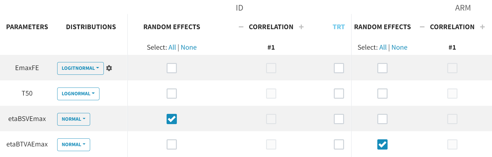
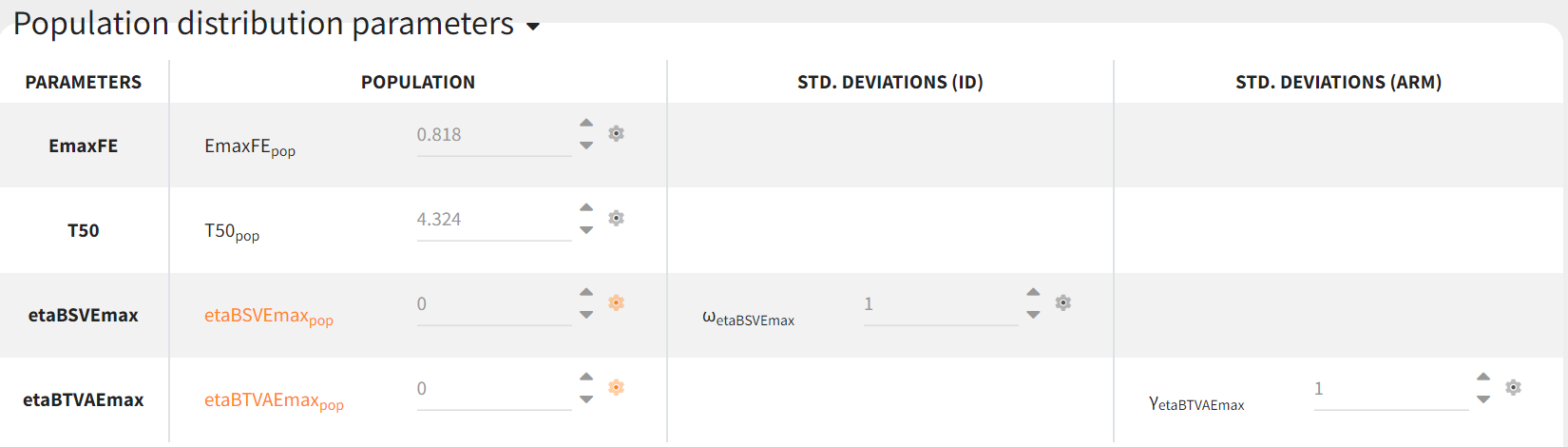
Since both etaBSVEmax and etaBTAVEmax are random effects parametrized as fixed effects with distribution
their means must be zero. This is done in the initial estimates tab, using the cog-wheel button to fix the respective initial estimates to zero.
Covariates
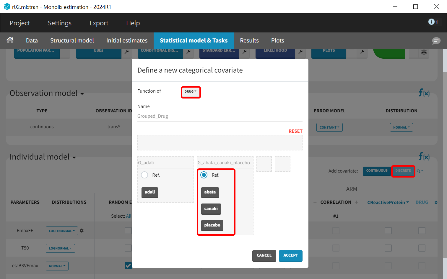
As a final step, we need to add DRUG as a covariate on EmaxFE and T50, in order to estimate one EmaxFE and one T50 value for each treatment (placebo, adalimumab, abatacept, and canakinumab). Before adding the DRUG column as covariate, we click on the add covariate / discrete button and create a new covariate called tDRUG for which placebo is the reference category:
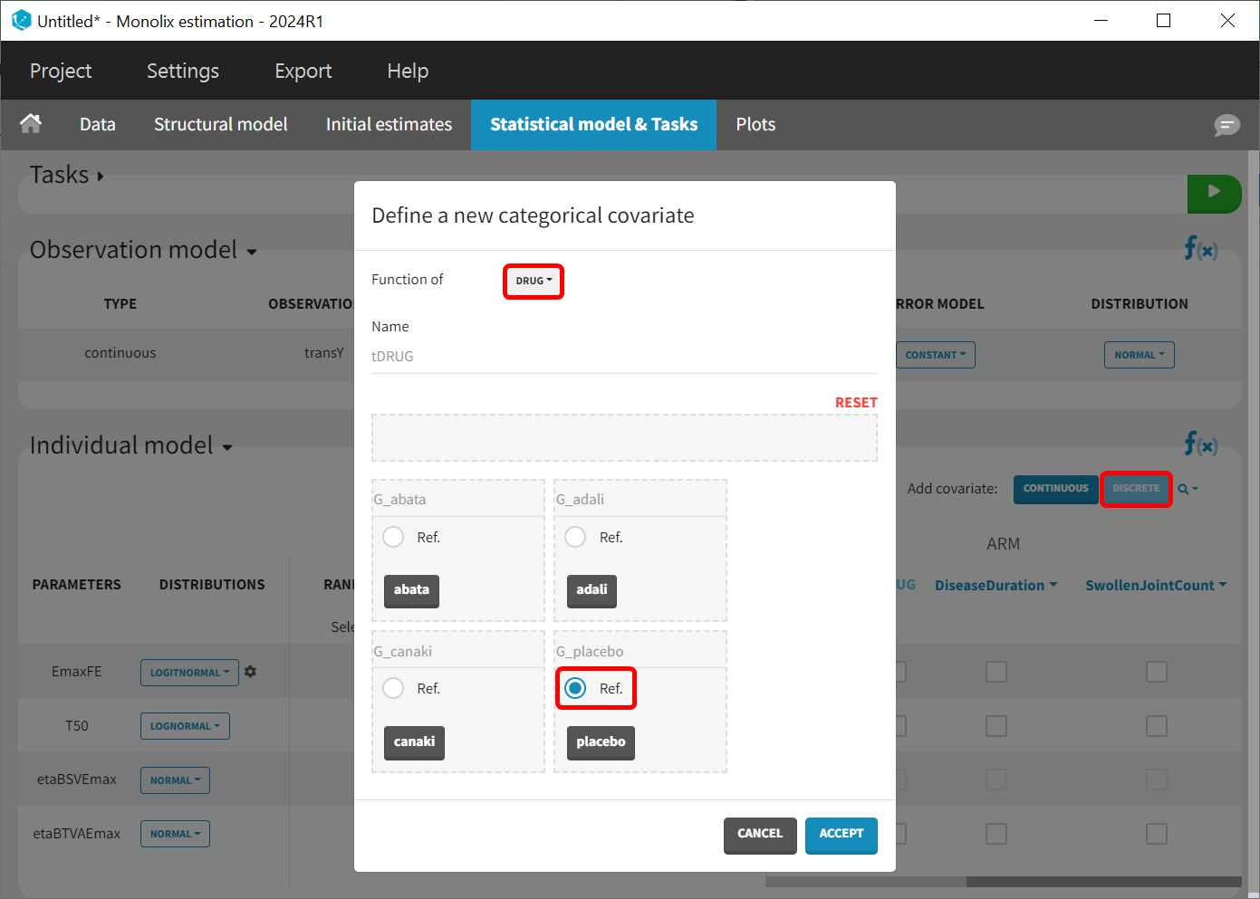
The newly created tDRUG is added on EmaxDE and T50. The other possible covariates will be investigated later.
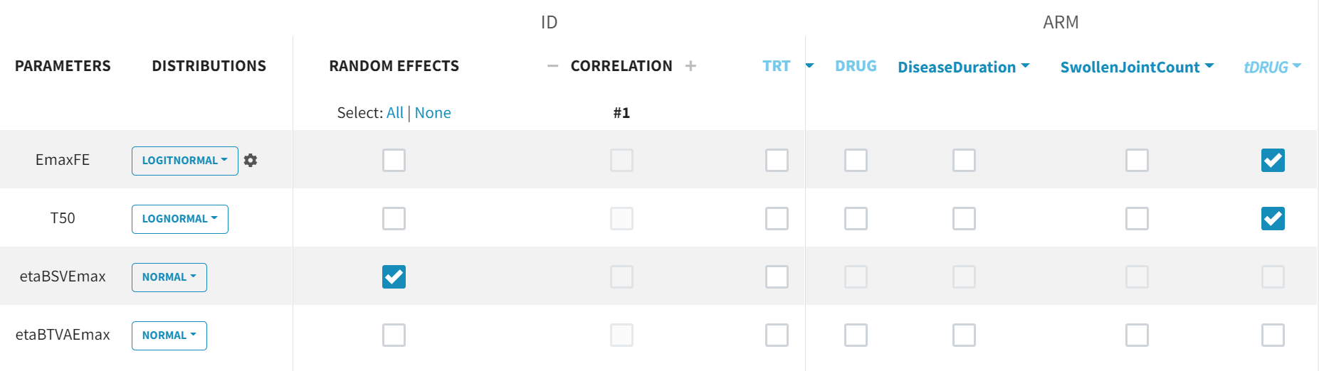
Summary view
Following this model set up, the Statistical model & Tasks tab should appear as shown below:
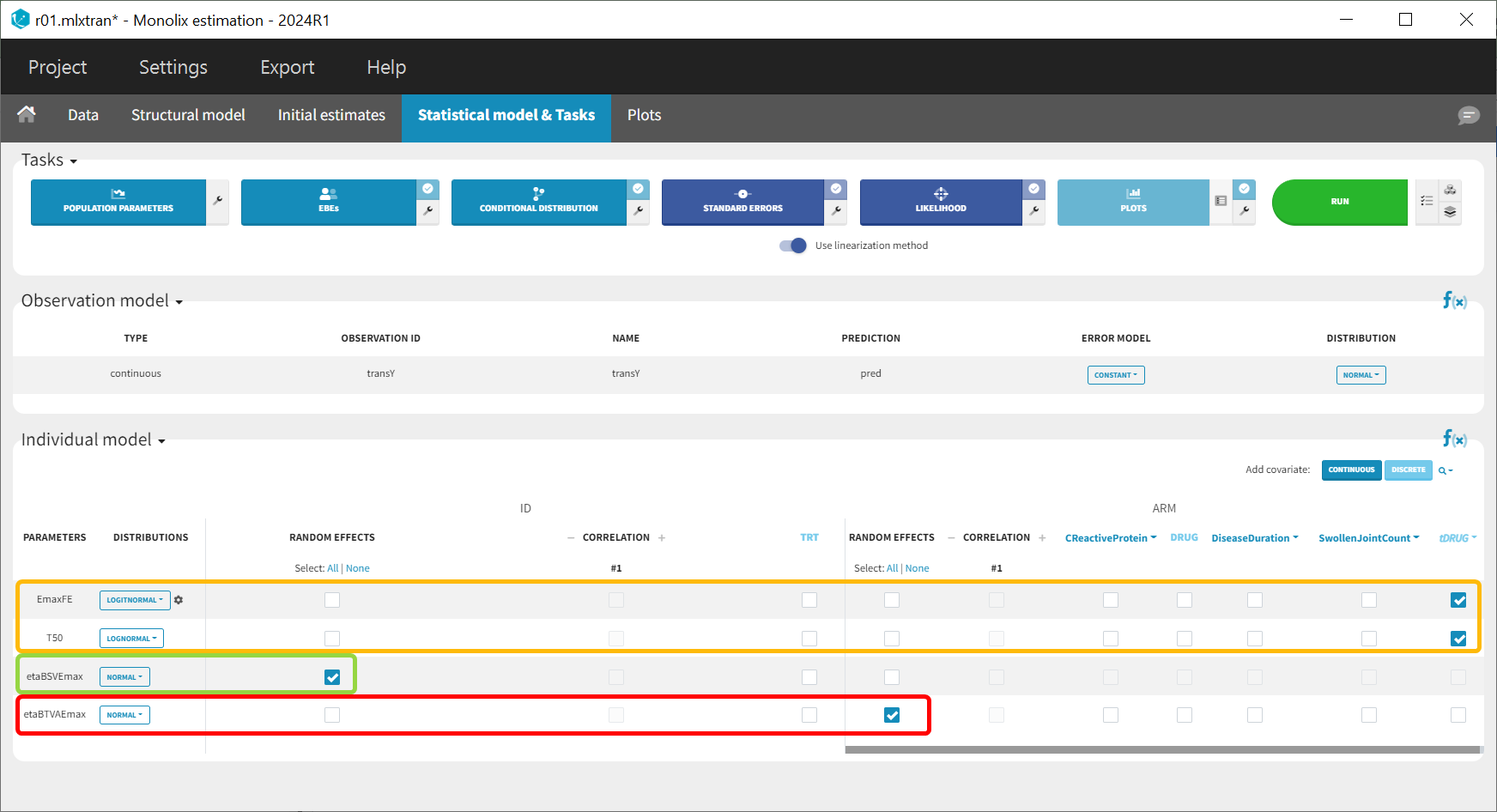
The model setup may be summarized as follows:
-
Tag column with N individuals per arm (Narm) as a regressor
-
Transform the observation column as follows:
-
Define the structural model
-
Set the observation error model to constant
-
Specify parameter distributions as appropriate for the structural model
-
Specify, for the eta parameters, the appropriate random effects (that is, BSV → study level only, BTAV → arm level only, also known as occasion) and also set their distributions to normal and fix their initial estimate (defined as population parameters) to zero
-
Add the drug as a covariate to the structural model parameters (consider transforming so placebo is reference)
Model development
Parameter estimation
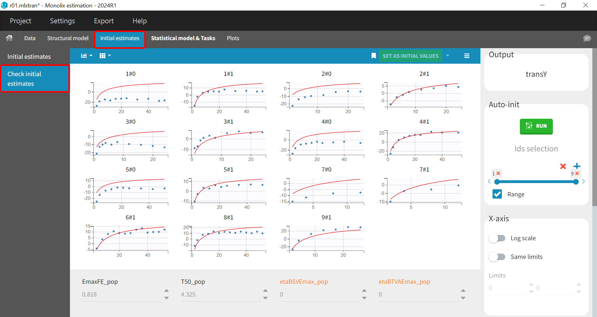
Finding initial values
Before starting the parameter estimation, we first try to find reasonable initial values. In the Initial estimates tab, Check initial estimates window, we can either set the initial values of the population parameters manually or run the auto-init function that finds the initial values for us, as in the image below. The red curve corresponds to the prediction with the estimated initial values, the blue dots correspond to the transY data.
Choosing the Settings
Before launching the parameter estimation task, be sure to save the project.
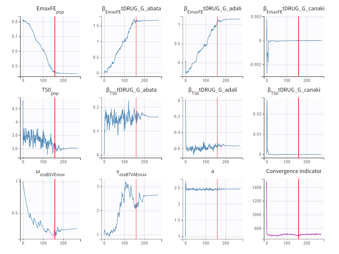
Next, we launch the parameter estimation task. After around 160 iterations, the stochastic approximation expectation maximization (SAEM) exploratory phase switches to the second phase, due to the automatic stopping criteria.
To assess the convergence, we can run the parameter estimation from different initial values and with a different random number sequence. To do so, we click on the “assessment” button and select “all” for the sensitivity on initial values. (The standard errors and likelihood tasks need to be checked as well.) Multiple estimations (five by default) will be done using varying seeds and randomly drawn initial values.
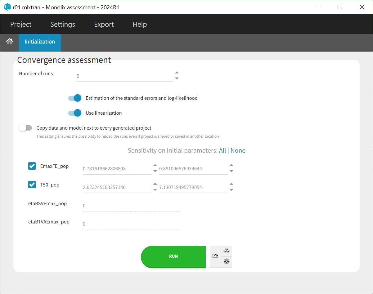
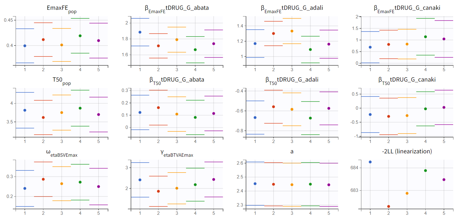
Convergence trajectories, final estimates, and repeated log-likelihood calculations can be examined to assess the robustness of the estimates.
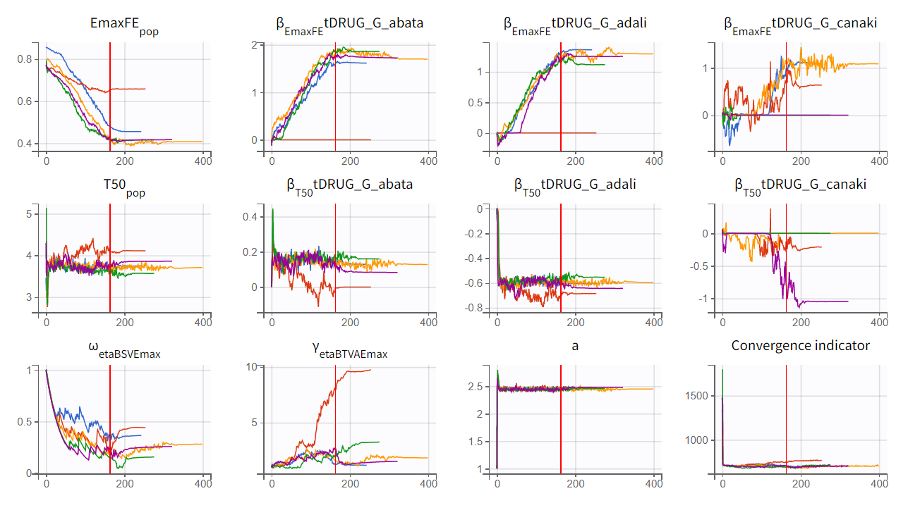
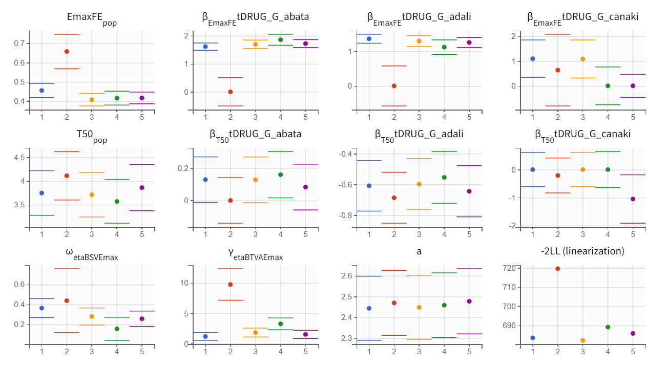
The colored lines in the first set of plots above show the trajectories of parameter estimates, while the colored horizontal lines in the second set of plots above show the SDs of the estimated values of each run. We see that the trajectories of many parameters vary a lot from run to run. Parameters without variability, such as EmaxFE, are usually harder to estimate. Indeed, parameters with and without variability are not estimated in the same way. The SAEM algorithm requires drawing parameter values from their marginal distribution, which is only possible for parameters with variability.
Several methods can be used to estimate the parameters without variability. By default, these parameters are optimized using the Nelder-Mead simplex algorithm. As the performance of this method seems insufficient in our case, we will try another method. In the SAEM settings (wrench icon next to the task “pop param” in the main window), three options are available in the “Methodology for parameters without variability” section as shown below:
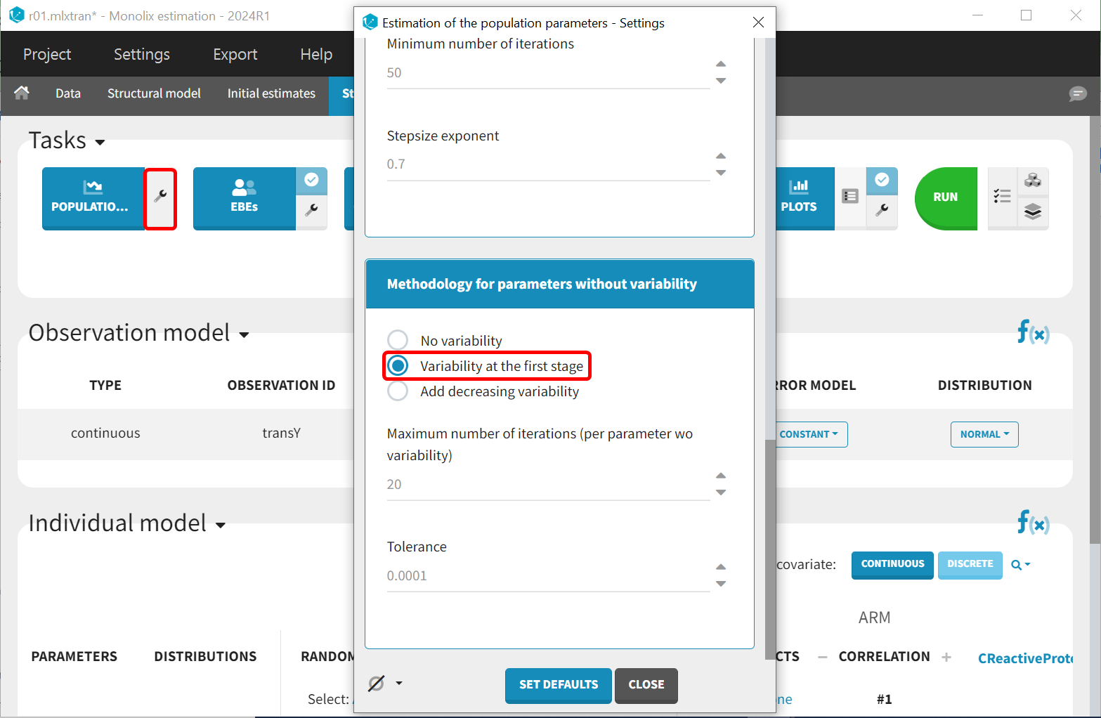
-
No variability (default): optimization via Nelder-Mead simplex algorithm
-
Variability in the first stage: during the first phase, artificial variability is added and progressively forced to zero. In the second phase, the Nelder-Mead simplex algorithm is used.
-
Add decreasing variability: artificial variability is added for these parameters, allowing estimation via SAEM. The variability is progressively forced to zero, such that at the end of the estimation proces, the parameter has no variability.
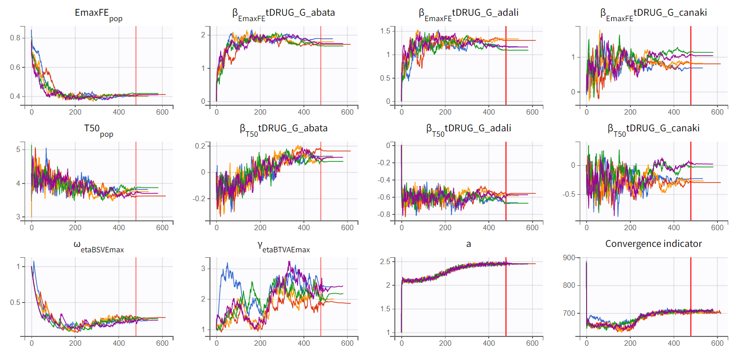
We choose the second option, “variability in the first stage” method, and launch the convergence assessment again (saving the project under a new name MBMA_r02_variability1stage.mlxtran). This time, the convergence is satisfactory. We no longer see parameters converging to multiple minima (for example, EmaxFE), and the likelihood is stable, varying less than 2 points across runs compared to over 15 points previously.
Results
These can be obtained by either of 2 ways:
-
From the *_rep folders containing the estimated values that have been generated during the convergence assessment.
-
Or, alternatively, redo the parameter estimation and the estimation of the Fisher information matrix (via linearization for instance) to get the standard errors.
Click on the Tests tab under Results. The point estimates in the Wald test, along with the associated p-values, represent the difference between the placebo and the other drug categories. A significant p-value indicates that the drug effect is statistically different from 0, meaning the covariate effect should be retained in the model.
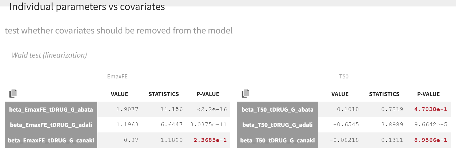
As indicated by the p-value (calculated via a Wald test), the Emax values for abatacept and adalimumab are significantly different from the Emax for placebo (with p-values much smaller than 0.05). On the other hand, given the data, the Emax value for canakinumab is not significantly different from placebo (p-value = 0.24). Note that when analyzing the richer individual data for canakinumab, the efficacy of canakinumab had been found significantly better than that of placebo (Alten R et al). The T50 values are similar for all compounds except adalimumab. Therefore, these drug covariate modalities can be pooled for the next model run (MBMA_r03_variability1stage_groupeddrug.mlxtran), creating a new covariate.
This new covariate will be included in the individual model as a covariate effect on T50, replacing the covariate tDRUG.
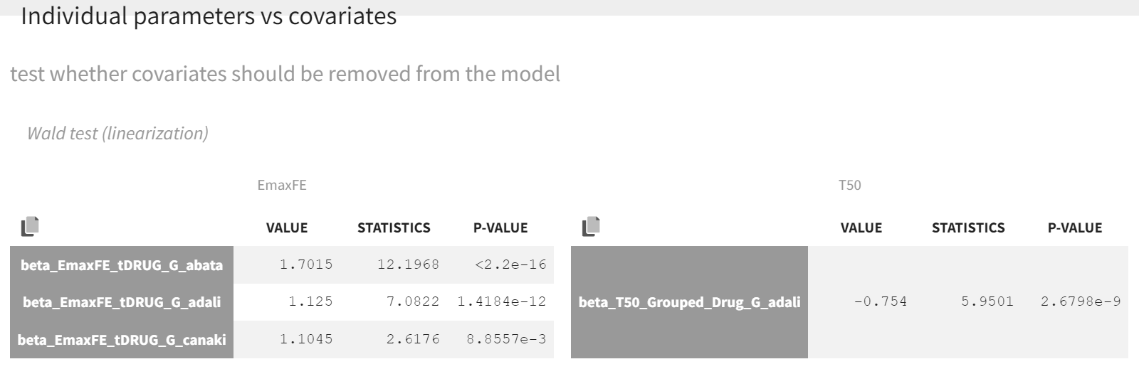
After launching the estimation tasks, the Wald test suggests that the new covariate should remain included in the individual model on T50, as the difference between adalimumab and canakinumab, abatacept, and placebo is significant.
The table below is displayed upon clicking on the POP.PARAMS tab under results.
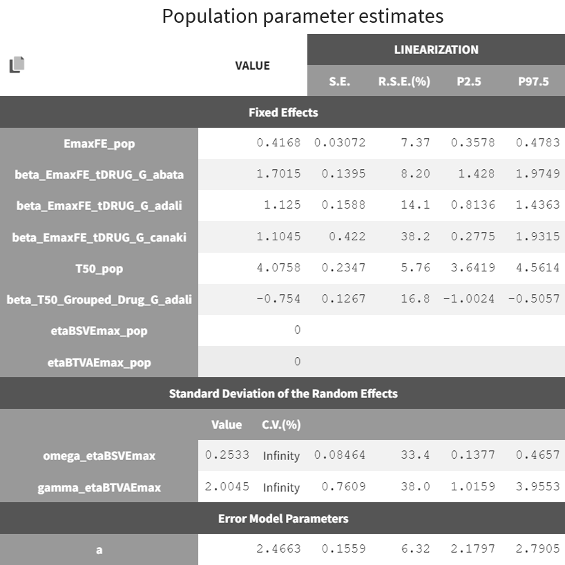
The BSV of Emax (omega_etaBSVEmax) is 0.25 and reflects the variability from study to study in the maximum percent of patients achieving ACR20 response. The BTAV is gamma_etaBTAVEmax = 2.00. While this may seem high, recall that in the model, the BTAV is expressed as follows:
For a typical number of individuals per arm of 200, dividing 2.00 by the square root of 200 yields the BTAV of Emax is approximately 0.14 (
). Note that after setting mean of the random effects BSVEmax_pop and BTAVEmax_pop equal to zero (in the GUI), we obtain infinity in the coefficient of variation (CV) expressed as a percent for omega_etaBSVEmax and gamma_etaBTAVEmax. The CV is defined as the quotient of the SD and the mean. The mean in the denominator being zero, the CV is computed as 1.79/0 → ∞.
Model diagnosis
We next estimate the study parameters (that is, individual parameters via EBSs task) and generate the graphics shown below. Based on these graphs, no model mis‑specification can be detected in the individual fits, observations versus predictions, residuals, or other graphics:
|
Individual fits 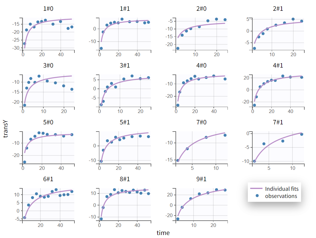
|
Observations vs predictions 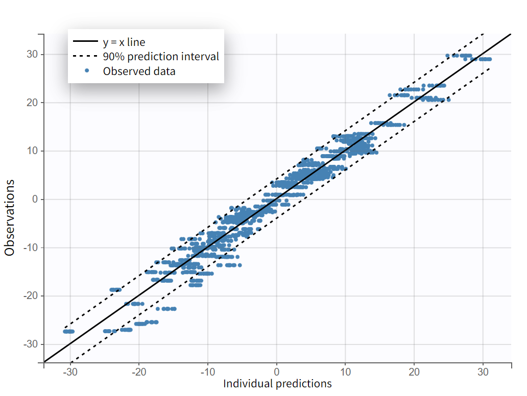
|
|---|
Note that all graphics in Monolix use the transformed observations and transformed predictions.
Untransformed plots for individual fits and the VPC can be created with the help of an R script available for download here. This allows plotting on the more interpretable original scale, which for ACR20 is the percent of individuals achieving 20% improvement.
|
Untransformed individual fits 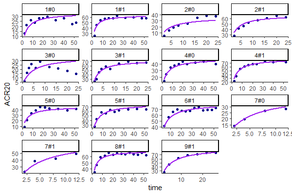
|
Untransformed VPC 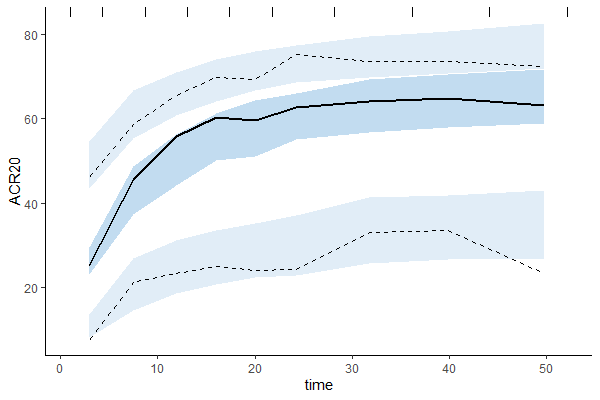
|
|---|
Alternative models
One could also try a more complex model including BSV and BTAV on T50. We leave this investigation as hands-on for the reader. The results are the following: the difference in Akaike information criterion (AIC) and Bayesian information criterion (BIC) between the 2 models is small and some standard errors of the more complex model are unidentifiable. Thus, we decided to keep the simpler model reported above.
Covariate Search
The BSV originates from the different inclusion criteria from study to study. To try to explain part of this variability, we can test by adding the studied population characteristics as covariates. The available population characteristics are the mean number of swollen joints, the mean C-reactive protein level, and the mean disease duration.
As these covariates differ between arms, they appear in the IOV window. To center the distribution of covariates around a typical value, we first transform the covariates using a reference value:
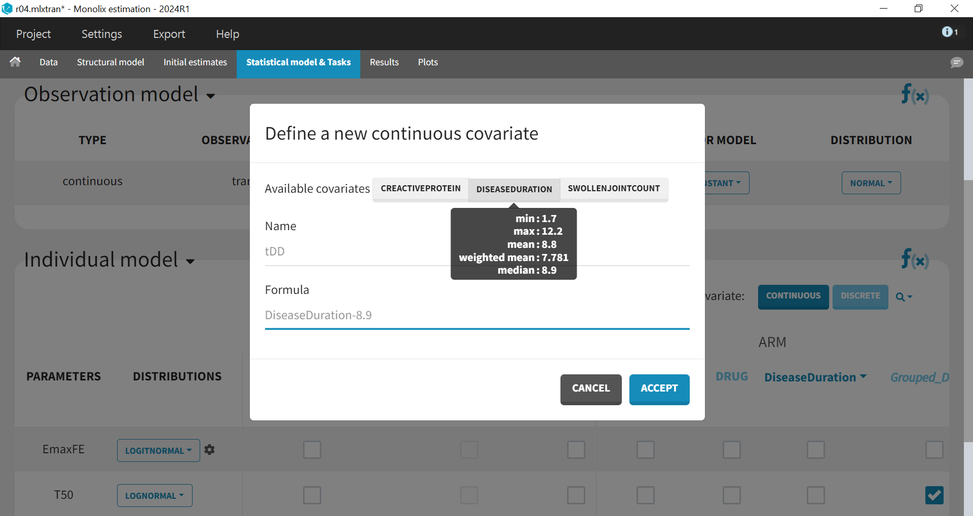
The covariates can be included one by one in the model on the Emax parameter as an example of a forward covariate model development approach. We can either assess their significance using a Wald test (p-value in the result file, calculated with the Fisher Information Matrix Task), or a likelihood ratio. The advantage of the Wald test is that it requires only 1 model to be estimated (the model with the covariate) while the likelihood ratio requires both models (with and without covariate) to be estimated.
In this case study, a backward approach has been employed, where all the covariates are included in the model on Emax simultaneously, followed by an evaluation to determine whether any covariates should be excluded (run04.mlxtran). The p-values from the Wald test assessing whether the beta coefficients are zero are as follows:
-
Disease duration: p-value=0.28 (not significant)
-
C-reactive protein level: p-value=0.75 (not significant)
-
Swollen joint count: p-value=0.14 (not significant)
The likelihood ratio test also indicates that none of these covariates is significant; therefore, they will not be included in the model.
Final model
The final model has an Emax structural model, with between study and between treatment arm variability on Emax, and no variability on T50. No covariates are included on these parameters.
The fixed effect EmaxFE incorporates the drug effect tDrug, reflecting all four drug modalities (abatacept, adalimumab, and canakinumab, and placebo), with placebo set as the reference drug.
For the parameter T50, a drug covariate effect is also included; however, the drug covariate has been regrouped to consist of only two modalities (adalimumab and adalimumab/canakinumab/placebo).
The final run is available in the materials (see the top of the page) and is named MBMA_r03_variability1stage_groupeddrug.mlxtran.
Simulations for decision support
Comparison of Canakinumab Efficacy With Drugs on the Market
Now, we would like to use the developed model to compare the efficacy of canakinumab with that of abatacept and adalimumab. Is there a chance that canakinumab is more effective? To answer this question, we will perform simulations using the simulation application Simulx.
To compare the true efficacy of canakinumab (over an infinitely large population) with abatacept and adalimumab, we could simply compare the Emax values. However, the Emax estimates are estimated with uncertainty, and this uncertainty should be taken into account. Thus, we will perform a large number of simulations for the three treatments, drawing the Emax population value from its uncertainty distribution. The BSV, BTAV, and residual error will be ignored (that is, set to zero) because we want to consider an infinitely large population to focus on the “true efficacy.” Thus, we are taking into account the error in estimating the EmaxFF_pop parameter (in the population parameters result table) and ignoring other sources of uncertainty at this time.
In order to run simulations, we need to export the final project from Monolix to Simulx as shown below:
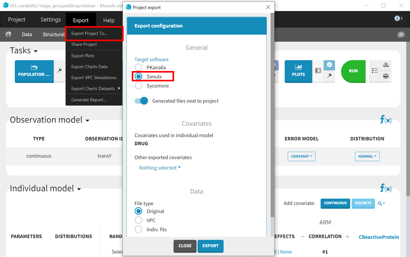
All the information contained in the Monolix project will be transferred to Simulx. This includes the model (both structural and statistical parts), estimated population parameter values and their uncertainty distribution, and original design of the dataset used in Monolix (number of individuals, treatments, covariates, observation times, etc.). Elements containing this information are generated automatically in the “Definition” tab of the new Simulx project. It is possible to use these elements to set up a simulation in the “Simulation” tab or to create new elements to define a new simulation scenario.
Among the elements created automatically is the occasion structure imported from the Monolix dataset. The first step is to delete this occasion element, as it’s not needed for these simulations. Recall the occasions are used for the BTAV which we decided to set to zero to compare true efficacy. Go to the “Definition” tab, click “OCCASIONS,” and then click on the “DELETE” button.
To compare the efficacy of canakinumab versus abatacept and adalimumab, we will simulate the value of ACR20 over 52 weeks in 4 different scenarios (that is, simulation groups) corresponding to canakinumab, abatacept, adalimumab, and also placebo.
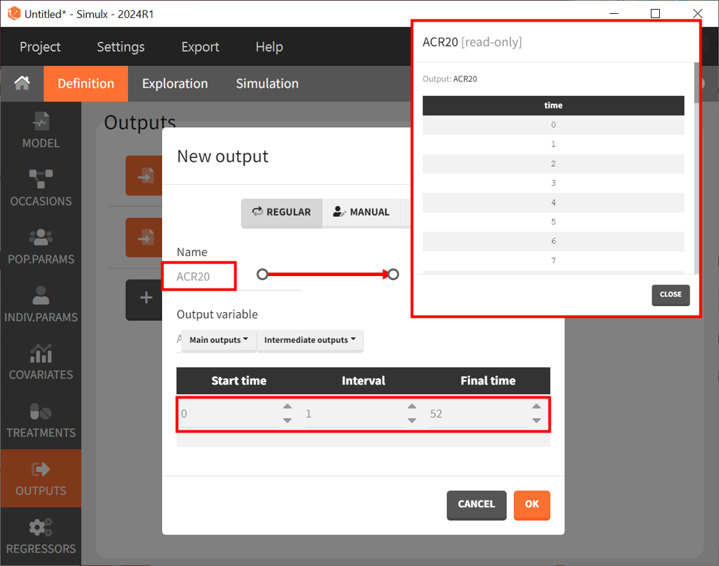
Next, let’s define the output. In Monolix, we were working with the transformed prediction of ACR20 because of the constraints on the error model. Here, we ignore the error model and concentrate on the model prediction so we can directly output the (untransformed) ACR20 for each week.
The definition of the output variable against which we will assess the efficacy of the treatments looks like this. We output ACR20 weekly on a regular grid from time zero to week 52.
Then, we need to define the treatments given, which appear in the model as a categorical covariate. This can be done directly in the “COVARIATES” tab. We need to define four different elements, each corresponding to one of the four treatments we want to simulate.
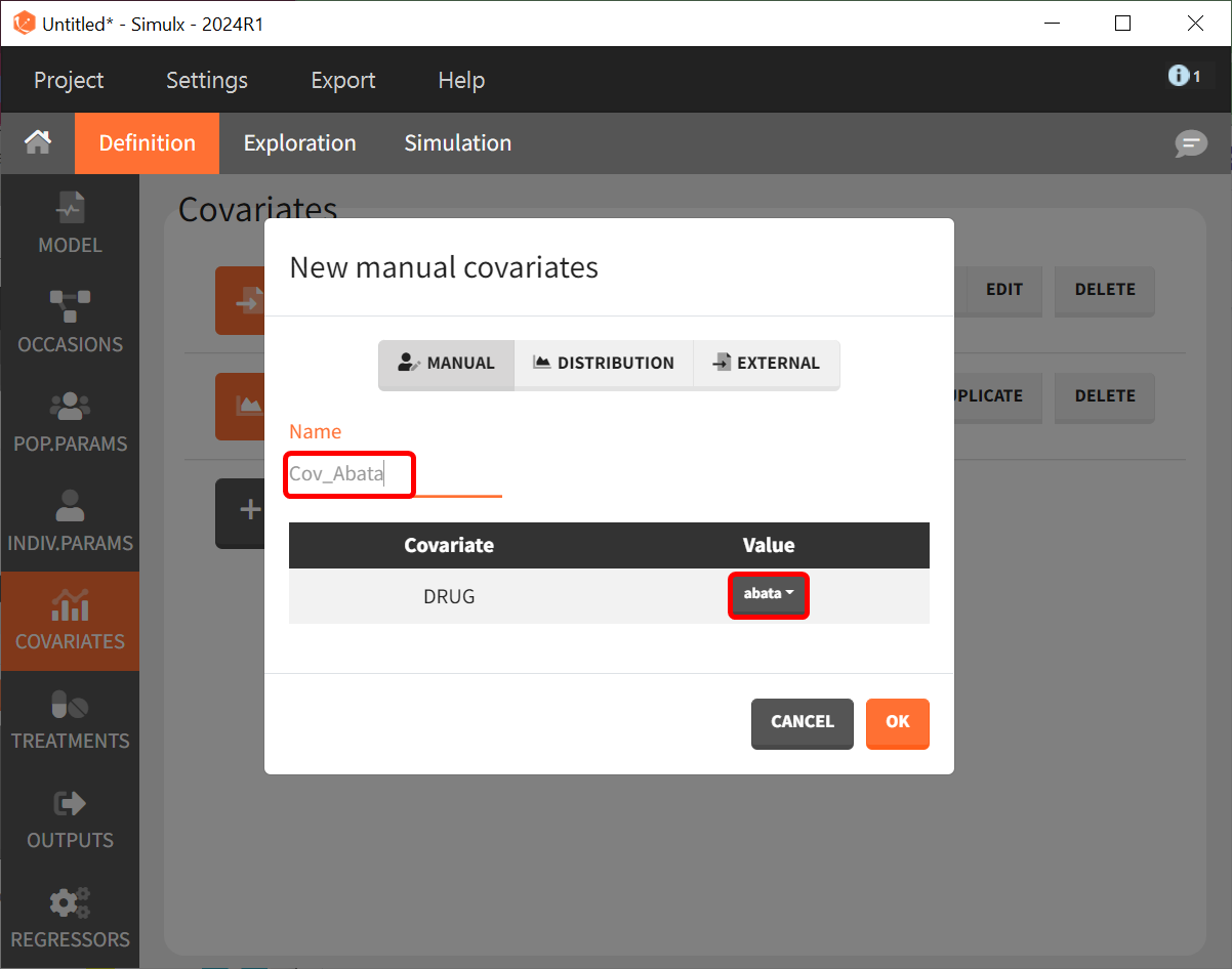
The definition of the other treatments (that is, Cov_drugname) is made analogously to the screenshot above with the appropriate label assigned and the corresponding drug selected from the dropdown in the “Value” column.
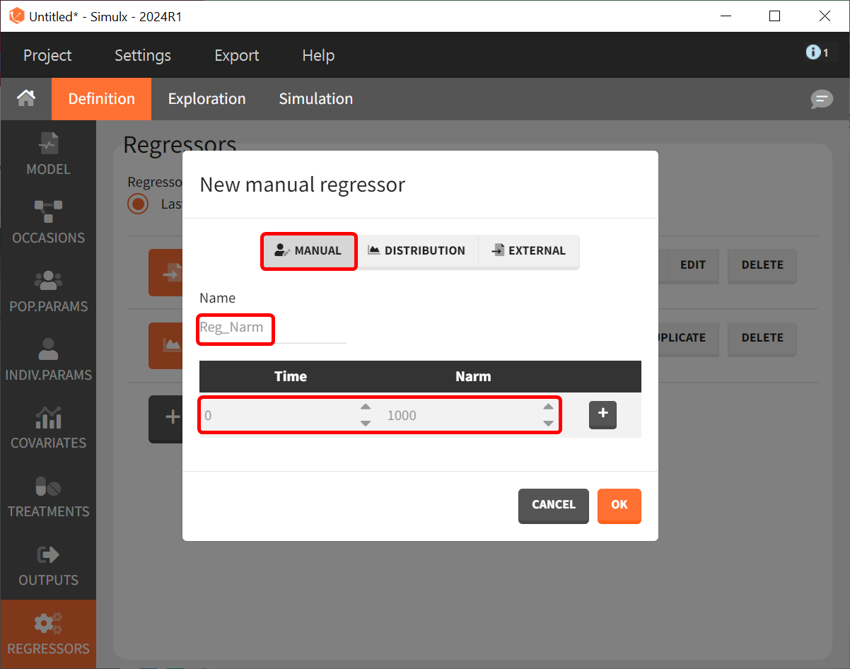
Lastly, we define a regressor representing the number of individuals per study. Later, we will see that this information needs to be defined since it was used in the model but will actually not influence the simulations because the BTAV and residual error are ignored.
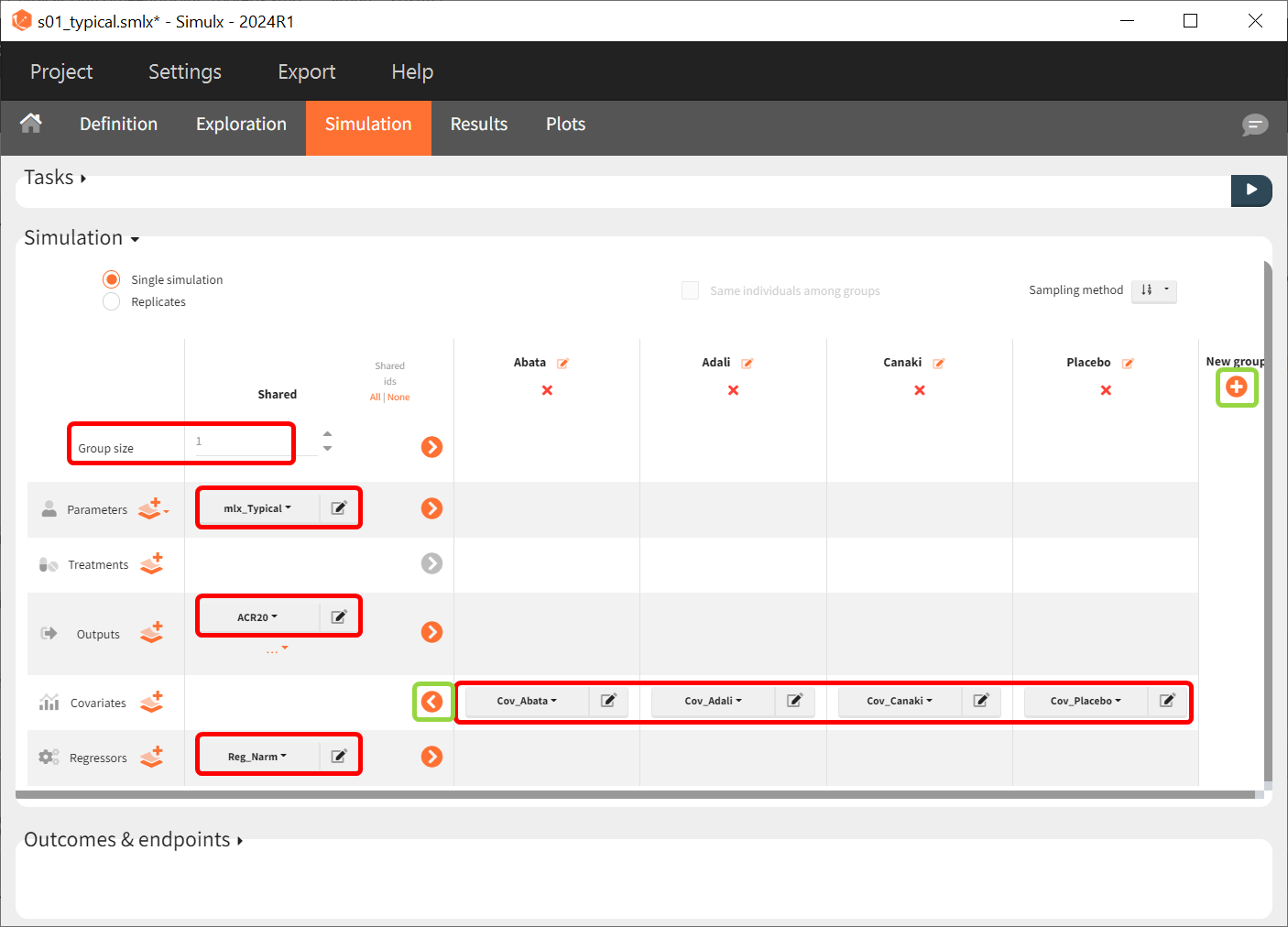
After defining the output, regressor, and treatment variables, we move to the the simulation tab. As an initial step, we will simulate the value of ACR20 for each treatment using the estimated Emax and T50 values and ignoring the uncertainty. Thus, we define four individuals (that is, studies), one with each treatment.
We set the group size to 1 since we want to simulate only one study per treatment. For parameter, we select mlx_Typical (available starting from version 2023). This element contains the population parameters estimated by Monolix, but with the SDs of the random effects set equal to zero. This allows us to simulate a typical study, ignoring the BSV and BTAV. For the output variable, we set the above-defined (untransformed) ACR20 vector. After clicking on the plus under “New group” to add more simulation groups, the previously defined covariates can be set as for each of the four simulation groups (note that we don’t use a standard treatment element due to how we set up our model to estimate the treatment effect from the covariate).
As regressor, we set the element Reg_Narm defined previously. In theory, the number of individuals in the treatment arms determines the BTAV. When the number of individuals goes to infinity, meaning Narm → ∞, the variability converges to zero, meaning etaBTAV/√Narm → 0. Since we want to describe an ideal scenario, we can set the number of individuals very high. However, we have chosen the element mlx_Typical for the parameter values for the simulation, which already sets the random effects (etaBSV and etaBTAV) and their SD equal to zero. Thus, in practice, Reg_Narm has no effect on the simulation.
After saving the project and then running the simulation, the “Output distribution” tab of the Plot section shows the response curves of the four treatment groups shown in four subplots. To combine the curves into a single plot, “Merged splits” can be used in the “STRATIFY” panel. In addition, by turning on the legend in the plot settings and optionally modifying the colors of the treatment arms in the “STRATIFY” tab, we obtain the following plot:
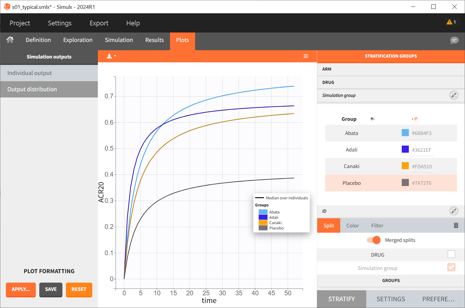
The simulation shown in this plot gives a first idea of the efficacy of canakinumab (orange curve) compared to the other treatments.
By defining outcomes and endpoints, this can be quantified.

We define a new outcome for ACR20 at the last time point, t = 52. The endpoint can use the arithmetic, geometric mean, or median within each simulation group. But this does not matter as we simulate only one study per group, so the endpoint will be equal to the outcome. We then choose to compare the groups using a direct comparison of the ACR20 values and using canakinumab as the reference group. Given that each treatment group has only one simulated study, no statistical comparison is possible, and we use a direct comparison. Since the efficacy of canakinumab will be compared with treatments already on the market, we set the tested difference to be ‘< 0.’ If the result is negative, canakinumab is considered more effective; for ‘= 0,’ it is considered equivalent (at the last time point) and, for ‘> 0,’ it is considered less effective. Written as a formula, we expect the following to be true for a successful experiment outcome:
The formula is analogous for the treatments abatacept and placebo compared to canakinumab.
After defining the outcomes and endpoints, save the project under a new name. Only the Outcome & Endpoint task needs to be executed; the simulations do not need to be rerun.
Under “Results,” selecting the SIMULATION tab on the left shows summary tables of the simulations per treatment arm, as well as a list of the individual parameters. The ENDPOINTS tab includes the arithmetic mean of ACR20 at the last time point, t = 52. The “StandardDeviation” column of the ENDPOINTS [TABLE] tab (or row of the ENDPOINTS [SUMMARY] tab), shows NaN (not a number) since we have set the sample size, which corresponds to the number of studies, to 1. In the GROUP COMPARISON tab, you can find the calculated mean difference of the treatment arms versus the reference treatment canakinumab. The “SUCCESS” column indicates whether the comparison can be interpreted as successful. If the difference is < 0, a green check mark appears in the column, if not, a black cross appears.
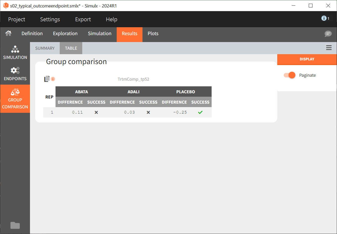
We see that the mean difference between abatacept and canakinumab, as well as adalimumab and canakinumab, respectively, is positive. This means that for the two treatment groups, the ACR20 value for abatacept or adalimumab was higher than for canakinumab at week 52. This suggests that, in the ideal case we simulated (infinitely large population), canakinumab is less effective than these two treatments already on the market. In the placebo versus canakinumab comparison, however, we see a negative difference, which is also consistent with the above plot of the effect curve. Canakinumab has a higher ACR20 value at week 52 than the placebo group. Therefore, we can conclude that canakinumab performs better than the placebo, which was expected.
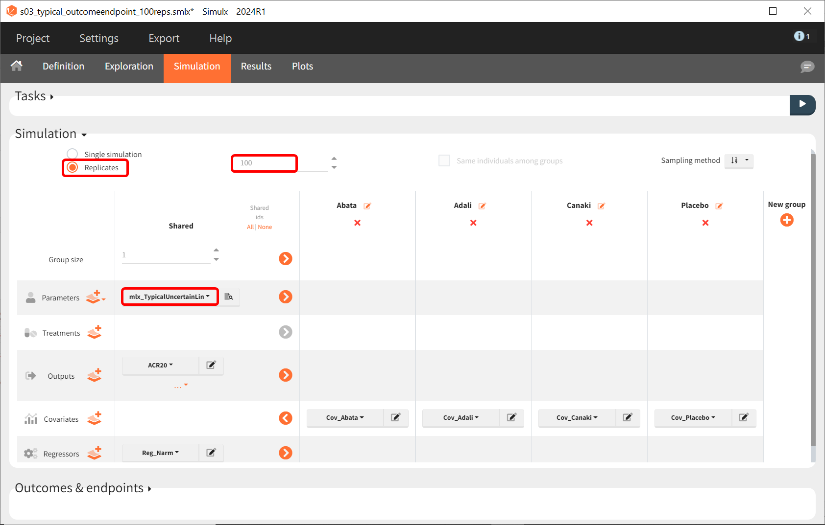
Next, we would like to calculate a prediction interval for the true effect, taking into account the uncertainty of the population parameters estimated by Monolix. To do so, we save the Simulx project under a new name and make the following changes to the simulation settings:
-
Create 100 replicates of the scenario
-
Change the population parameters from mlx_Typical to mlx_TypicalUncertain (available starting with version 2023). This element contains the estimated variance‑covariance matrix of the population parameters estimated by Monolix with SDs of the random effects set to 0. It enables simulation of a typical individual (meaning a study) with different population parameter values for each replicate, such that the uncertainty of population parameters is propagated to the predictions.
The defined outcomes and endpoints remain unchanged. The goal is to assess the impact on the success criterion when the scenario is repeated 100 times using different sets of population parameters.
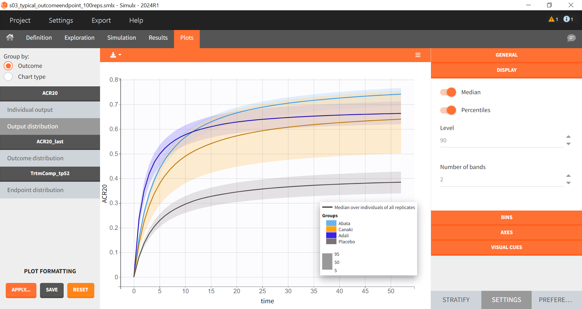
The output distribution plot shows the response curve, but now with the percentiles of the simulated data calculated from all replicates. The “number of bands” under DISPLAY in the settings tab can be set to 2 and the subplots merged to facilitate the comparison.
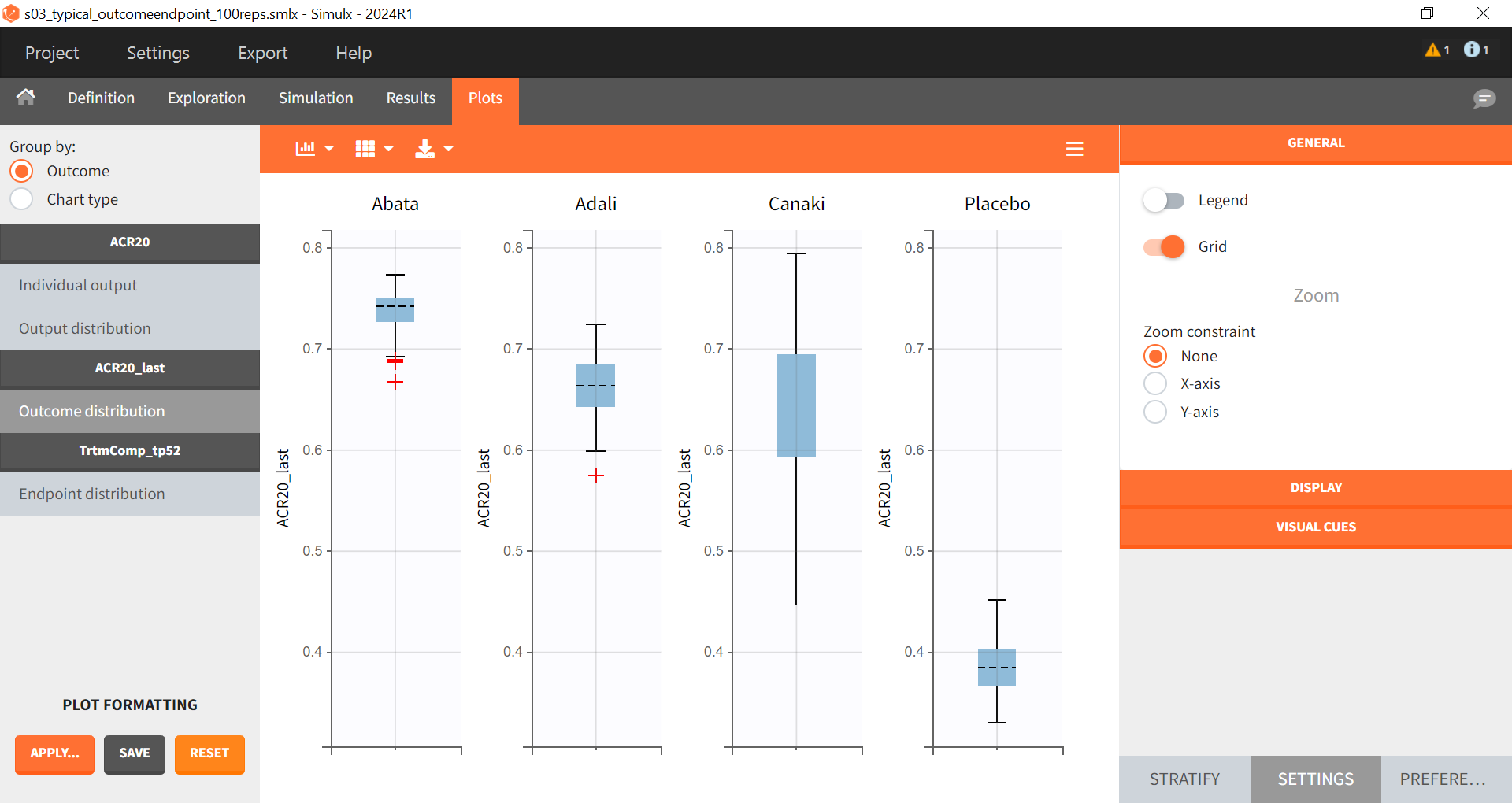
In the “Endpoint distribution” tab of the plots, we see the distribution of the replicates of ACR20 at week 52 across all four treatment groups. It is clear that the treatments with the active compounds are more effective than the placebo group. However, for 100 replicates, the median value of canakinumab is below the median values of abatacept and adalimumab.
Note: Canakinumab has wider percentile bands in the “Output distribution” plot as well longer box + whiskers in the “Endpoint distribution” boxplot. This is due to there being less data available compared to the other treatments. This leads to a larger uncertainty of the true effect of canakinumab in comparison to the other drugs.
If we go back to the Results section, we find similar tables to the previous simulation, but this time with results per replicate.

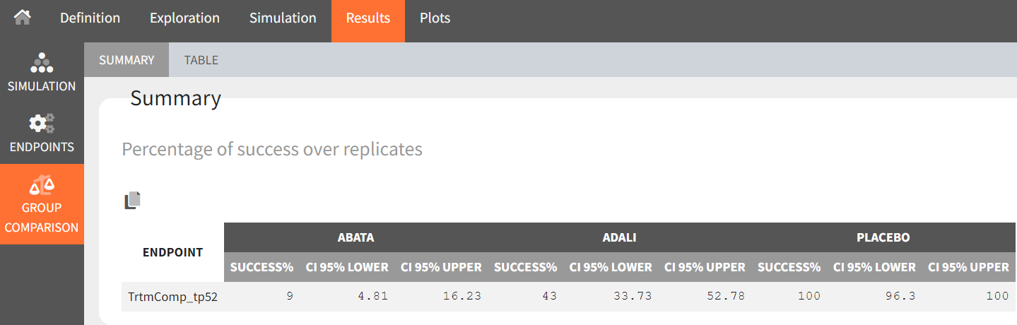
From the summary table, we can conclude that at time point, t = week 52, given the estimated population parameters:
-
Out of 100 repetitions, the comparison
was true only 9 times. Therefore we have a 9% chance that canakinumab performs better than abatacept.
-
Out of 100 repetitions, the comparison
was true only 43 times. Therefore we have a 43% chance that canakinumab performs better than adalimumab.
-
Out of 100 repetitions, the comparison
was true all 100 times. Therefore we have a 100% certainty that canakinumab performs better than the placebo.
This finding supported the decision to not continue with clinical development of canakinumab in RA, as reported in Demin I et al.
Conclusion
Model-informed drug development
Model based meta-analysis supports critical decisions during the drug development process. In the present case, the model has shown that chances are low that canakinumab performs better than two drugs already on the market. As a consequence, the development of this drug has been stopped, thus saving the high costs of Phase 3 clinical trials.
MBMA with Monolix and Simulx
This case study also aims at showing how Monolix and Simulx can be used to perform longitudinal model-based meta-analysis. Contrary to the usual parameter definition in Monolix, the weighting of the between treatment arm variability necessitates splitting the parameters into their fixed term and their BSV and BTAV terms and reformatting the parameter in the model file. Once the logic of this model formulation is understood, the model set-up becomes straightforward. The efficient SAEM algorithm for parameter estimation as well as the built-in plots then allow users to efficiently analyze, diagnose and improve the model.
The inter-operability between Monolix and Simulx also facilitates the transfer of the Monolix project to Simulx to easily define and run simulations.
Natural Extensions
In this case study, continuous, bounded data were used. Yet, the same procedure can be applied to other types of data such as count, categorical or time-to-event data.
Guidelines to Implement Your Own MBMA Model
Setting Up Your Dataset
The data set should usually contain the following columns:
-
STUDY: index of the study/publication. It is equivalent to the ID column for individual-level data.
-
ARM: index of the arm (preferably continuous integers starting at 0). There can be an arbitrary number of arms (for instance several treated arms with different doses) and the order doesn’t matter. This column will be used as equivalent to the occasion OCC column.
-
TIME: time of the observations
-
Y: observations at the study level (percentage, mean response, etc.)
-
transY: transformed observations, for which the residual error model is constant
-
Narm: number of individuals in the arm. Narm can vary over time. Alternatively, empirical standard error can be used instead. The variable to be used for weighting the observations should be tagged as a regressor in the structural model.
-
Covariates: continuous or categorical covariates that are characteristics of the study or of the arm. Covariates must be constant over arms (appear in IOV window) or over studies (appear in main window).
Frequent Questions About the Dataset
-
Can dropouts (i.e. a time-varying number of individuals per arm) be taken into account? Yes. This can be accounted for without difficulty as the number of subjects per arm (Narm) is passed as a regressor to the model file, a type that allows, by definition, variations over time. This is also applicable in case variance is used, since variance also accounts for the sample size.
-
Can there be several treated (or placebo) arms per study? Yes. The different arms of a study are distinguished by a ARM index. For a given study, one can have observations for ARM=0, then observations for ARM=1, then observations for ARM=2. The index number has no special meaning (for instance ARM=0 can be the treatment arm for study 1, and ARM=0 the placebo arm for study 2).
-
Why should I transform the observations? The observations must be transformed such that an error model from the drop-down menu in the GUI (constant, proportional, combined) can be used. In the example above, we applied two transformations. First, we use a logit transformation that enables bounded observations of the fractions of individuals reaching ACR20 to be mapped to the normal space, enabling, in turn, a normally distributed error term to be estimated. This transformation ensures that the prediction of the fraction of individuals achieving ACR20 remains within the 0-1 interval, even if the residual error term is large (note that the predictions need to be back transformed to be on the scale of the original ACR20 values, that is, is bounded within the 0-1 interval). Another example would be when predicting a mean concentration of glucose, we could use a log-transformation to ensure positive values. Second, we multiply each value by the square root of the number of individuals per arm. With this transformation, the SD of the error term is weighted for the number of individuals per arm and thus is consistent across all studies and treatment arms, regardless of the number of individuals per arm. Note that we could also weight by the empirical standard error instead of square root of the number of individuals per arm. This has the advantage of using the SD from the underlying studies, rather than assuming it is constant across studies.
Setting Up Your Model
The setup of your project can be done in four steps:
-
Split the parameters in several terms
-
Transform parameters as appropriate
-
Set the parameter definition in the Monolix interface
-
Back transform the transformation of the prediction
Frequently Asked Questions on Setting Up the Model
-
Why should I split a parameter into several terms? The SD of the BTAV term must usually be weighted by the square root of the number of individuals per arm; this term must be handled as a separate parameter and added to the fixed effect within the model file. This step is not possible in the GUI. Moreover, the fixed effect and its BSV random effects may also be split depending on the covariate definition.
-
How do I know in how many terms should I split my parameter?
-
If all covariates of interest are constant over studies: In this case, the parameters can be split into a (fixed effect + BSV) term and a (BTAV) term. The model file would, for instance, be (for a logit distributed parameter):
-
[LONGITUDINAL]

input = {paramFE_BSV, etaBTAVparam, Narm}

Narm = {use=regressor}

EQUATION:

tparam = logit(paramFE_BSV)

tparamRE = tparam + etaBTAVparam/sqrt(Narm)

paramRE = 1 / (1+ exp(-tparamRE))
Impact on the interface: In the GUI, paramFE_BSV would have both a fixed effect and a BSV random effect. Covariates can be added on this parameter in the main window. The etaBTAVparam fixed effect should be fixed to zero, the BSV disabled and the BTAV in the IOV part enabled.
-
If one covariate of interest is not constant over studies: This was the case for our case study, where the DRUG covariates were constant across arms but not studies. In this scenario, the parameters must be split into a fixed effect term, a BSV term, and a BTAV term. The model file could be structured as follows (for a logit-distributed parameter):
[LONGITUDINAL]

input = {paramFE, etaBSVparam, etaBTAVparam, Narm}

Narm = {use=regressor}

EQUATION:

tparam = logit(paramFE)

tparamRE = tparam + etaBSVparam + etaBTAVparam/sqrt(Narm)

paramRE = 1 / (1+ exp(-tparamRE))
Impact on the interface: In the GUI, paramFE has only a fixed effect (BSV random effect must be disabled in the variance-covariance matrix). Covariates can be added on this parameter in the IOV window. The fixed effect value of etaBSVparam and etaBTAVparam should be fixed to zero, the BSV disabled, and the BTAV in the IOV part enabled.
-
Why shouldn’t I add covariates on the etaBTAVparam in the IOV window? Covariates can be added on etaBTAVparam in the IOV window. Yet, because the value of etaBTAVparam will be divided by the square root of the number of individuals in the model file, the covariate values in the dataset must be transformed to compensate. This may not always be feasible:
-
If the covariate is categorical (as the DRUG for example), it is not possible to compensate and thus the user should not add the covariate on the etaBTAVparam in the GUI. Splitting into three terms is needed.
-
If the covariate is continuous (weight for example), it is possible to compensate. Thus, if you add the covariates on the etaBTAVparam in the GUI, the covariate column in the data set must be multiplied by
beforehand. This has a drawback, however this model has less parameters without variability and may thus converge more easily.
-
-
How should I transform the parameter depending on its distribution? Depending on the original parameter distribution, the parameter must first be transformed as in the following cases:
-
For a parameter with a normal distribution, called paramN for example, we could do the following:
-
; no transformation on paramN as it is normally distributed
tparamN = paramN
; adding the random effects (RE) due to between-study and between arm variability, on the transformed parameter
tparamNRE = tparamN + etaBSVparamN + etaBTAVparamN/sqrt(Narm)
; no back transformation as tparamNRE already has a normal distribution
paramNRE = tparamNRE
Note that the two transformations are not necessary but there for clarity of the code.
-
For a parameter with a log-normal distribution, called paramLog for example (or T50 in the case study), we could do the following:
; transformation from paramLog (log-normally distributed) to tparamLog (normally distributed)
tparamLog  = log(paramLog)
; adding the random effects (RE) due to between-study and between arm variability, on the transformed parameter
tparamLogRE = tparamLog  + etaBSVparamLog + etaBTAVparamLog/sqrt(Narm)
; transformation back to have paramLogRE with a log-normal distribution
paramLogRE = exp(tparamLogRE)
-
For a parameter with a logit-normal distribution on [0,1], called paramLogit for example (or Emax in the case study), we could do the following:
; transformation from paramLogit (logit-normally distributed) to tparamLogit (normally distributed)
tparamLogit  = logit(paramLogit)
; adding the random effects (RE) due to between-study and between arm variability, on the transformed parameter
tparamLogitRE = tparamLogit  + etaBSVparamLogit + etaBTAVparamLogit/sqrt(Narm)
; transformation back to have paramLogitRE with a logit-normal distribution
paramLogitRE = 1 / (1+ exp(-tparamLogitRE))
-
For a parameter with a generalized logit-normal distribution on [a,b], called paramLogit for example, we could do the following:
; transformation from paramLogit (logit-normally distributed in ]a,b[) to tparamLogit (normally distributed)
tparamLogit  = log((paramLogit-a)/(b-paramLogit))
; adding the random effects (RE) due to between-study and between arm variability, on the transformed parameter
tparamLogitRE = tparamLogit + etaBSVparamLogit + etaBTAVparamLogit/sqrt(Narm)
; transformation back to have paramLogitRE with a logit-normal distribution in ]a,b[
paramLogitRE =(b * exp(tparamLogitRE) + a)/ (1+ exp(tparamLogitRE))
-
How do I set up the GUI? Depending which option has been chosen, the fixed effects and/or the BSV random effects and/or the BTAV random effects of the model parameters (representing one or several terms of the full parameter) must be fixed to 0. Random effects can be disabled by clicking on the RANDOM EFFECTS column and fixed effects by choosing “fixed” after a click in the initial estimates tab.
-
Why and how do I transform the prediction? The model prediction must be transformed in the same way as the observations of the data set, using the column Narm passed as regressor or a column representing the empirical standard error.
Parameter estimation
The splitting of the parameters into several terms may introduce model parameters without variability. These parameters cannot be estimated using the main SAEM routine, but instead are optimized using alternative routines. Several of them are available in Monolix, under the settings of SAEM. If the default method leads to poor convergence, we recommend testing other methods.
Model evaluation
All graphics are displayed using the transformed observations and predictions. These are the correct quantities to diagnose the model using the “Observation versus prediction” and “Scatter plot of the residuals”, and “distribution of the residuals” plots. For the individuals fits and VPC, it may also be interesting to look at the non-transformed observations and predictions. The analysis as well as the generation of the plots can be redone in R using the simulx function of the RsSimulx package or the lixoft connectors. The other diagnostic plots (“Individual parameters vs covariates”, “Distribution over the individual parameters”, “Distribution of the random effects”, and “Correlation of the random effects”) are not influenced by the transformation of the data.
Literature examples
The following is a selection of recent articles implementing an MBMA using Monolix:
|
Reference Link |
Manuscript title |
|---|---|
|
Population-based meta-analysis of bortezomib exposure–response relationships in multiple myeloma patients |
|
|
Longitudinal model-based meta-analysis of lung function response to support phase III study design in Chinese patients with asthma |
|
|
Postmarketing assessment of antibody–drug conjugates: Proof-of-concept using model-based meta-analysis and a clinical utility index approach |
|
|
Population pharmacokinetics of erlotinib in patients with non-small cell lung cancer (NSCLC): A model-based meta-analysis |
|
|
A model-based meta-analysis of pembrolizumab effects on patient-reported quality of life: Advancing patient-centered oncology drug development |
There is also a published tutorial including this case study with additional examples:
C. Bracis, A. Taneja, Y. K. Lyauk, H. Barcomb, A. de la Peña, and G. Cellière, “ Model-Based Meta-Analysis With MonolixSuite: A Tutorial for Longitudinal Categorical and Continuous Data,” CPT: Pharmacometrics & Systems Pharmacology 15, no. 2 (2026): e70158, https://doi.org/10.1002/psp4.70158. PMID: 41347637