A TTE model for the NCCTG lung cancer study

Download data set only | Download all Monolix and Simulx project files | Download Simulx R script

This time-to-event case study represents a detailed modeling and simulation workflow using MonolixSuite applications. It is recommended to read before the Introduction to TTE data and library of models in Monolix.

Another case study on time-to-event data is also available: Case study on veteran lung cancer data set

In this case study, we develop a model for the NCCTG survival data set and study the effect of covariates.

https://www.youtube.com/watch?v=FkKhCzfA68c

Introduction

The North Central Cancer Treatment Group (NCCTG) data set records the survival of 228 patients with advanced lung cancer, together with assessments of the patients performance status measured either by the physician and by the patients themselves. The goal of the study was to determine whether patients self-assessment could provide prognostic information complementary to the physician’s assessment.
This data set has been originally presented and analyzed in:

Loprinzi et al. (1994). Prospective evaluation of prognostic variables from patient-completed questionnaires. North Central Cancer Treatment Group. Journal of Clinical Oncology : Official Journal of the American Society of Clinical Oncology, 12(3), 601–607.

This case study will test several parametric models to fit the dataset and assess the prognostic performance of the recorded covariates.

Data set visualization

The data set contains 228 patients, including 63 patients that are right censored (patients that left the study before their death). The original data set has been reformatted according to the data set formatting guidelines and includes both the starting time and the time of death or drop out.
To assess the importance of self performance assessment versus physician’s assessment, the following covariates have been recorded:

ecogPH: ECOG (Eastern Cooperative Oncology Group) performance status assessed by the physician, on a scale from 0 (fully active) to 5 (dead). For information on the scale, click here.
karnoPH: Karnofsky performance status, assessed by the physician, on a scale from 0 (dead) to 100 (completely healthy). More details about the scale can be found here.
karnoPAT: Karnofsky performance status, assessed by the patient
sex: sex of the patient (F for female, M for male)
age: age of the patient (years)

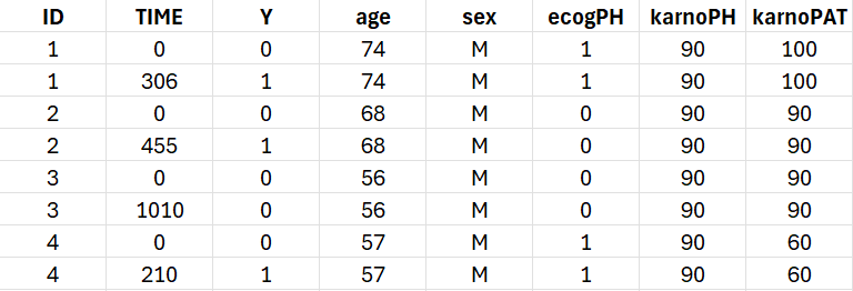
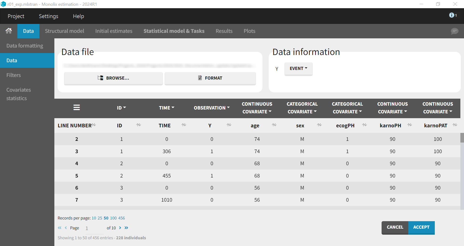
First, use Monolix to visualize the data set. After opening Monolix, start a new project and load the data, ensuring that covariates are assigned to the appropriate tags (continuous or categorical). In the Data Information section, specify that the data is of the EVENT type to visualize time-to-event data.

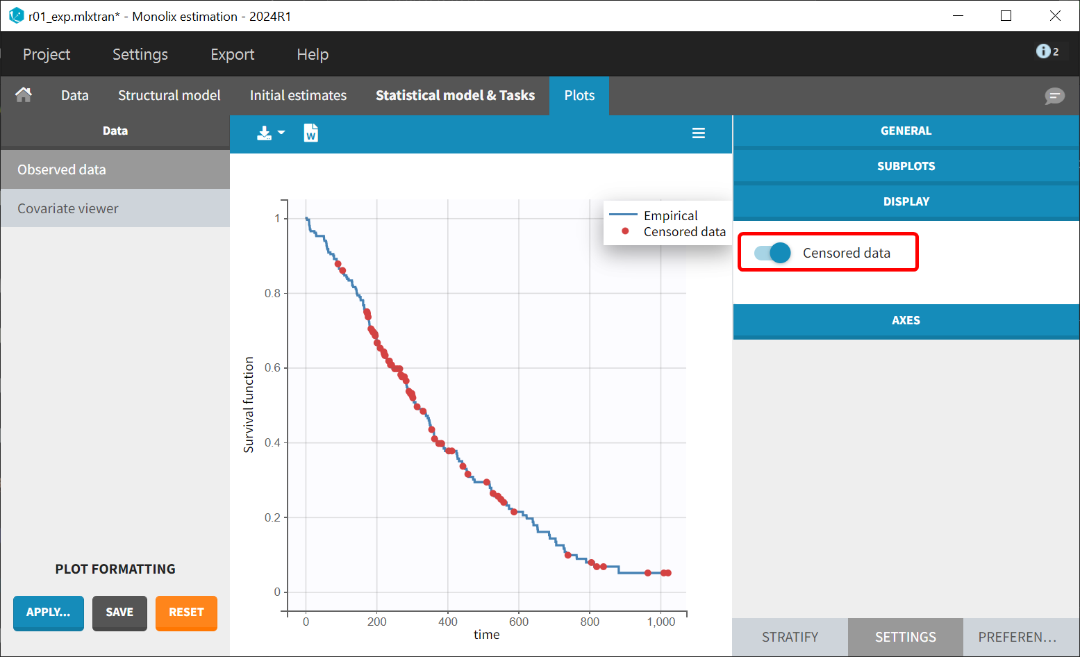
Once the dataset is accepted, the Kaplan-Meier (KM) estimate of the survival curve will appear in the Plots tab. In the “Settings” panel (right side), options are available to add the mean number of events curve and display censored data.

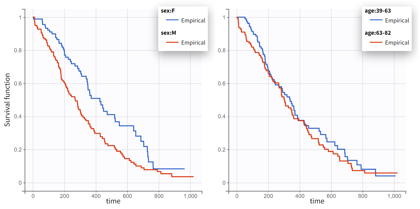
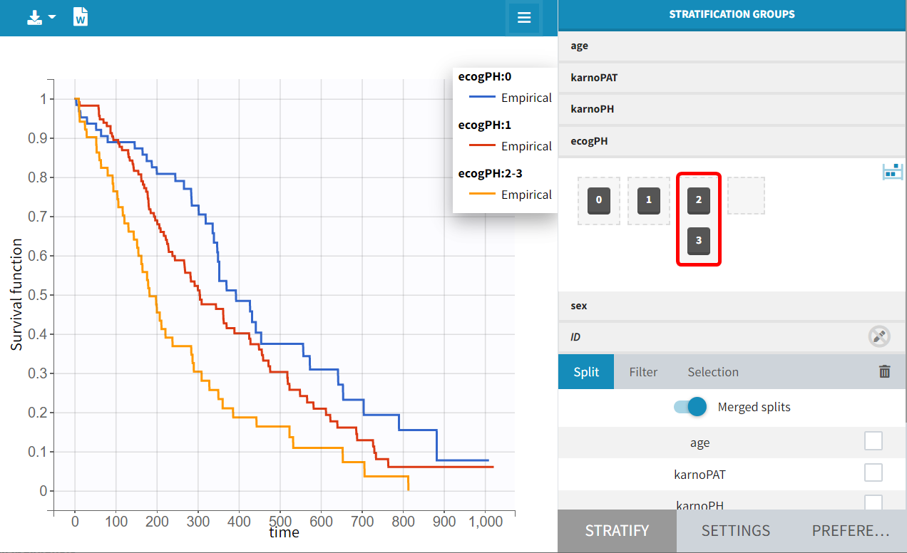
The Kaplan-Meier curve cannot be stratified by “coloring”, but you can split it and then a “merge” with a button that appears. It will merge the plots in one figure with different colors (fixed) for each curve. Add legend to visualize the assignment of colors to each stratification group.

Note that ECOG, karmoPH and karnoPAT are all performance scores and that they are probably strongly correlated.

In the Covariate Statistics section of the data tab, it can be seen that only one subject in the population has category 3 as the ECOG PH score:

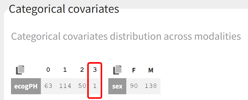
It can therefore be assumed that the score of this subject has a negligible impact on the population. Modalities 2 and 3 of the ECOG PH score can thus be pooled:

Modeling with Monolix

A model for this dataset will be developed to analyze which covariates have the highest prognostic performance. Within the MonolixSuite, only parametric models for time-to-event data are possible (no non-parametric or semi-parametric approaches).

Structural model

The development of the structural model begins by considering the typical shapes of common parametric survival models, as presented in the introduction to time-to-event modeling, along with the library of common TTE models. Based on the Kaplan-Meier curve visualization, models such as Weibull, log-logistic, gamma, or Gompertz could be appropriate. Each model is tested in turn by selecting the files with the extension "_singleEvent.txt" from the library.

For models with two parameters, it is common practice to assume that the shape parameter remains constant across individuals, while the scale parameter can vary between them. This inter-individual variability can be explained by the effect of covariates or random effects (often referred to as frailty models). Following this approach, random effects are disabled for the shape parameters ( and ) by adjusting the corresponding diagonal element of the variance-covariance matrix, while random effects are retained for the scale parameter . The default log-normal distributions are kept to ensure positive values for the parameters.

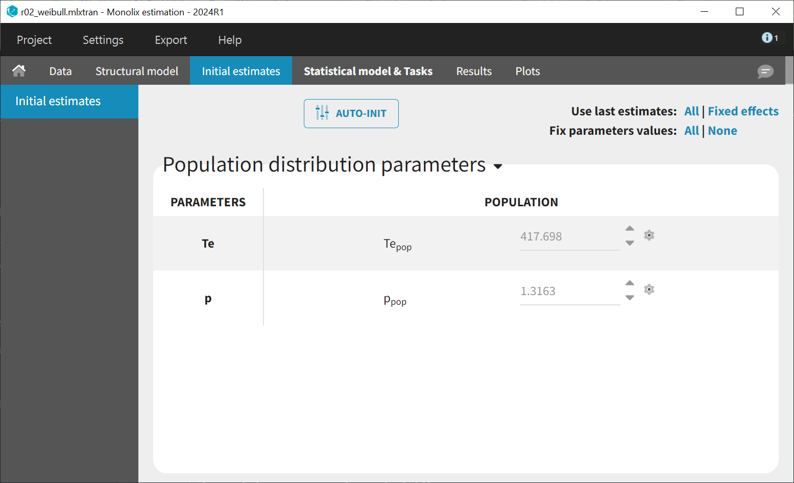
In each model, the scale parameter is represented by the characteristic time . Based on the Kaplan-Meier data visualization, an initial value of 300 is chosen, corresponding to a survival rate of around 50%. The shape parameter is initialized at 1, according to the typical value chart provided on the introduction page to TTE modelling. Starting from the Monolix2021R1 version, the auto-initialization is available also for time-to-event data.

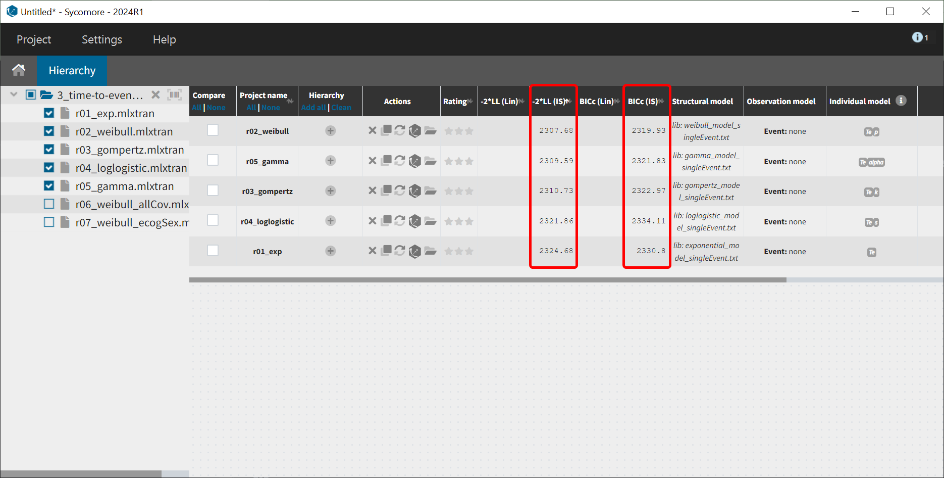
Next, the estimation tasks are launched for each structural model in turn: estimation of the population parameters, individual parameters, standard errors via the Fisher Information Matrix, log-likelihood estimation, and generation of graphics. The performance of each structural model can then be assessed and compared using the TTE graphics and log-likelihood values. A Sycomore project is used to organize and compare different models.

After each run, the VPC can be reviewed. A summary is presented below:

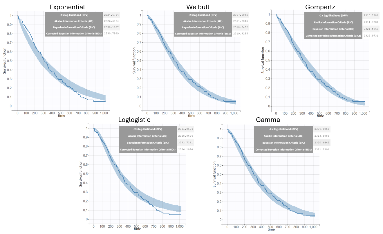
The "empirical" toggle in the VPC for time-to-event data refers to displaying the Kaplan-Meier survival curve based on the observed data. This shows the real survival behavior without model assumptions. The prediction interval with a 90% level reflects the range in which 90% of the model's simulated survival curves fall. If the empirical curve lies mostly within this interval, it suggests the model predictions align well with the observed data, indicating an acceptable model fit.

From a visual point of view, the exponential, log-logistic and gamma models can be excluded as they do not capture the shape of the KM curve. The Weibull and Gompertz models are satisfactory, with a slight preference for the Weibull model, as indicated by the BIC values. Therefore, the Weibull model is selected as the final structural model.

Covariate model

The investigation of covariates on the parameter focuses on explaining inter-individual variability. For educational purposes, covariate search will be conducted manually in a stepwise manner. In Monolix, using a backward covariate search approach is especially powerful. Indeed, after having calculated the s.e, a Wald test is performed to test the significance of each covariate. Thus it is sufficient to estimate the parameters of the model including all covariates relationships to get a p-value for each relationship, without having to estimate the submodels with one covariate relationship less. Following this strategy, we will estimate the model with all available covariates on and stepwise remove the less significant relationship, until all remaining covariates are significant. The AIC and BIC will also be monitored in parallel.

Since only one subject has an ecogPH score of 3, this modality can be combined with the ecogPH score 2 modality into a single category. To add the covariate, use the ‘Discrete' button to create a new categorical covariate, assigning both '2' and '3' to the reference group 'G_2_3’.

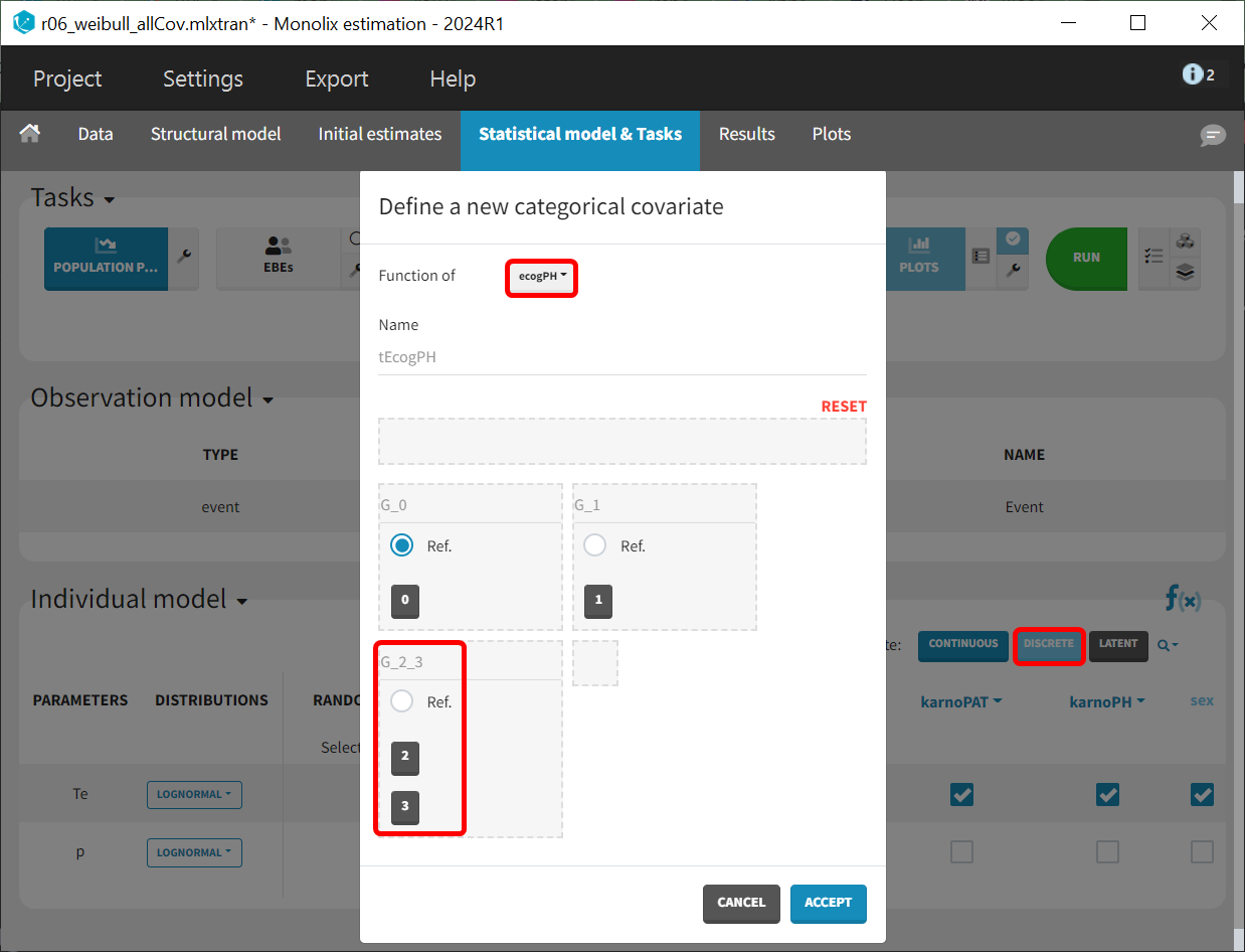
All covariates are added to the Te parameter in the "Covariate model" section. This corresponds to defining a model for that includes the influence of all selected covariates:

The table below summarizes the stepwise covariate removal, based on the p-values, and information criteria AIC, BICc and OFV:

The models with (sex, tEcogPH, karnoPAT) and (sex, tEcogPH) have similar AIC and BIC values. However, the model including (sex, tEcogPH, karnoPAT) has a high condition number (around 300). The condition number, which is the ratio of the maximal and minimal eigenvalues, indicates whether the model may be over-parameterized. A low condition number (i.e., less than 100) suggests a well-specified model. Due to this, the (sex, tecogPH) model is preferred.

Final model

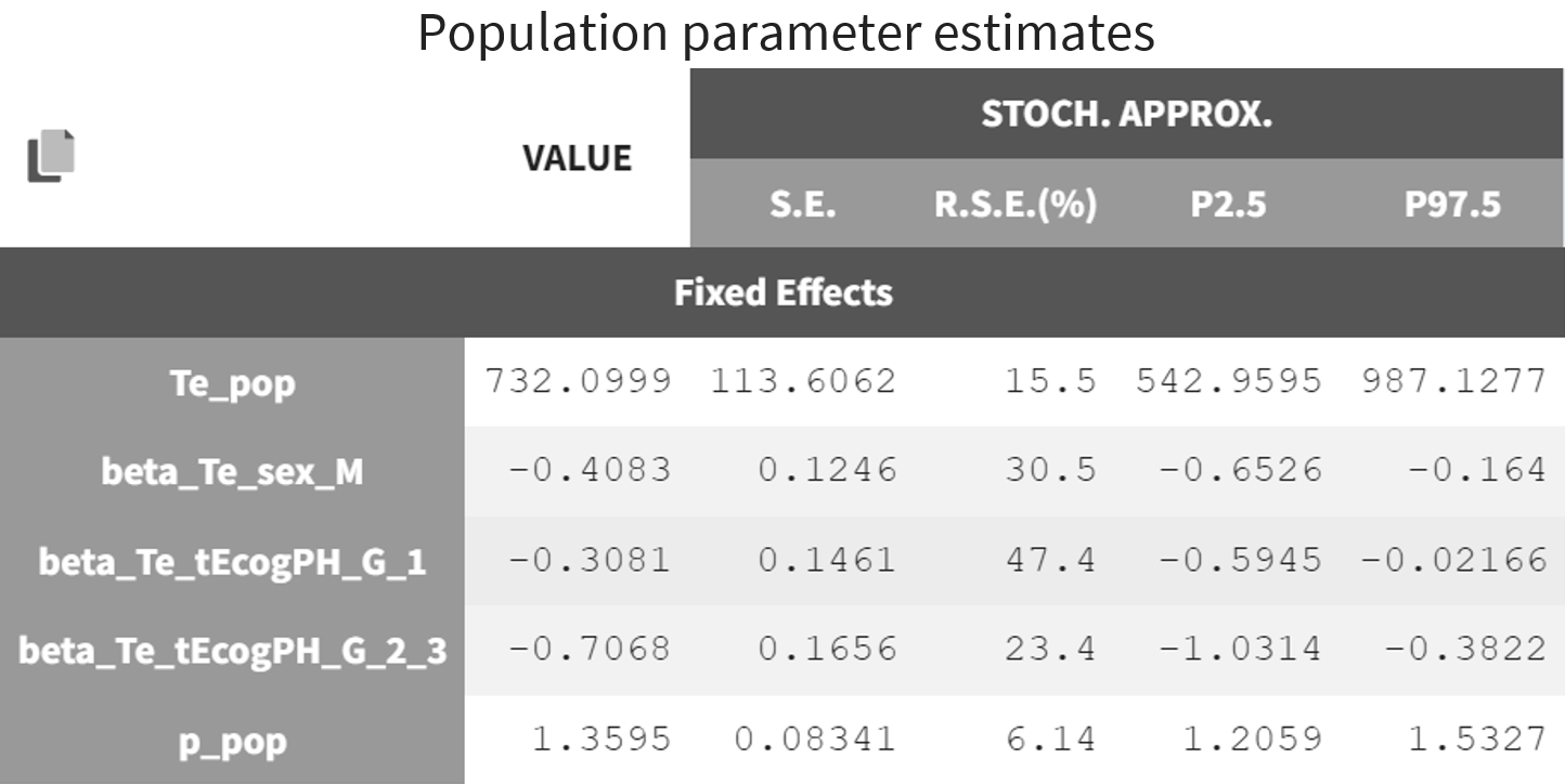
The final model incorporates a Weibull structural model with sex and ecogPH as covariates on the scale parameter Te. The model improvement when karnoPAT is included in addition to ecogPH is very small indicating that a self-assessment of the performance status by the patient permits only a slightly better prognosis, compared to using the physicians ECOG performance status evaluation only. In the original study including more patients and different types of cancer, the value of patient self-assessment was higher.

The estimated population parameters are displayed below. The r.s.e are reasonable.

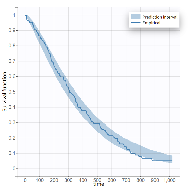
The 90% prediction interval for the KM curve shows that the data is properly captured. The other graphics do not hint at any model mis-specification.

For a given sex and ecogPH score, the typical hazard and associated Weibull survival can be calculated analytically:

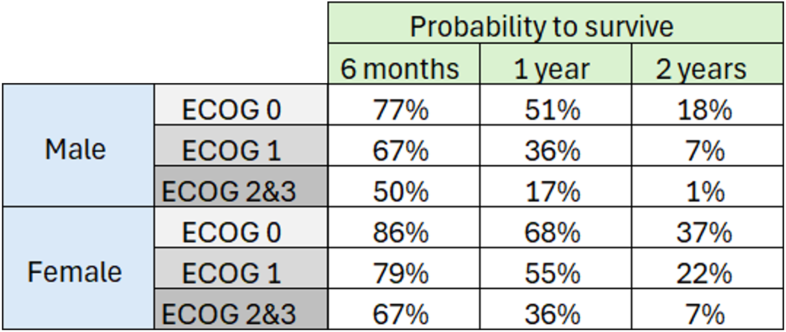
Using the survival function, it is possible to determine the probability of surviving for at least 6 months (182.5 days), 1 year (365.25 days), or 2 years (730.5 days), based on sex and ECOG score:

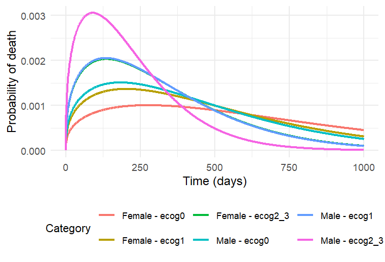
The probability density function of the death event can be calculated analytically as the product of the hazard and survival functions, based on a given sex and ECOG score. The probability of death over time for three different cases is shown below. This plot can also be interpreted as the distribution of death times in each of the three sub-populations.

Simulations using Simulx GUI

The model developed in Monolix can be applied to simulate new populations. In this case, three new patient cohorts with different covariate profiles compared to the original data set will be simulated. The three cohorts have the following characteristics:

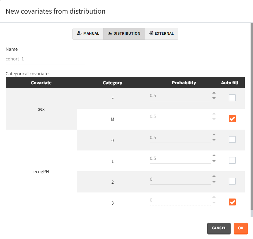
cohort 1: 50% male / 50% female, good ECOG scores (0 or 1)
cohort 2: 50% male / 50% female, poorer ECOG scores (2 or 3)
cohort 3: 90% male / 10% female, good ECOG score (0 and 1)

To simulate these three cohorts, the final Monolix project is imported into Simulx. The model (structural and statistical), parameters (population and individual), outputs and covariates are imported from the Monolix project and its data set. In the Simulation tab of Simulx, the default scenario corresponds to re-simulating a dataset used in the Monolix project.

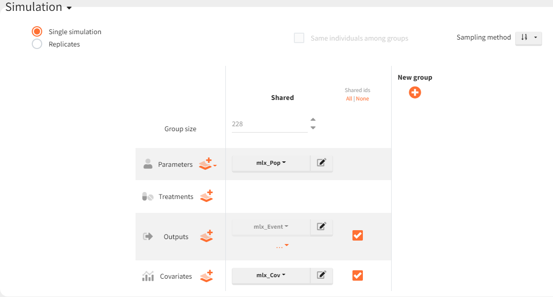
To simulate new cohorts, three groups are created, each with a specific covariate element corresponding to the defined characteristics. For instance, cohort 1 is configured as follows:

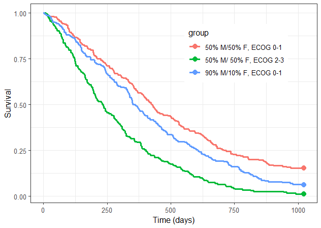
After running the scenario, the three Kaplan-Meier curves (one per group) are displayed in the Plots tab.

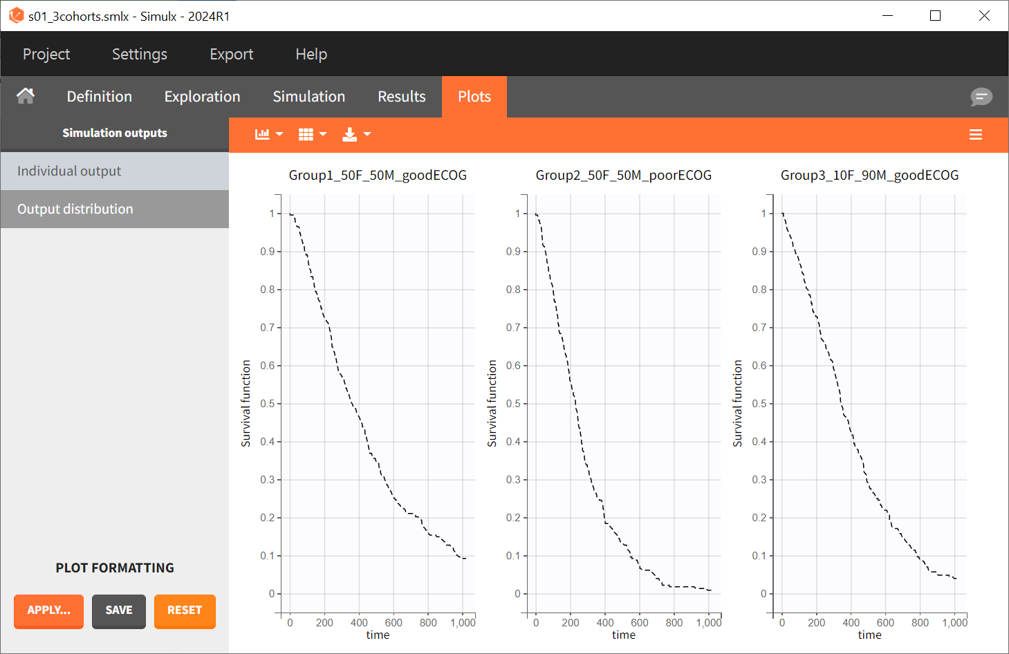
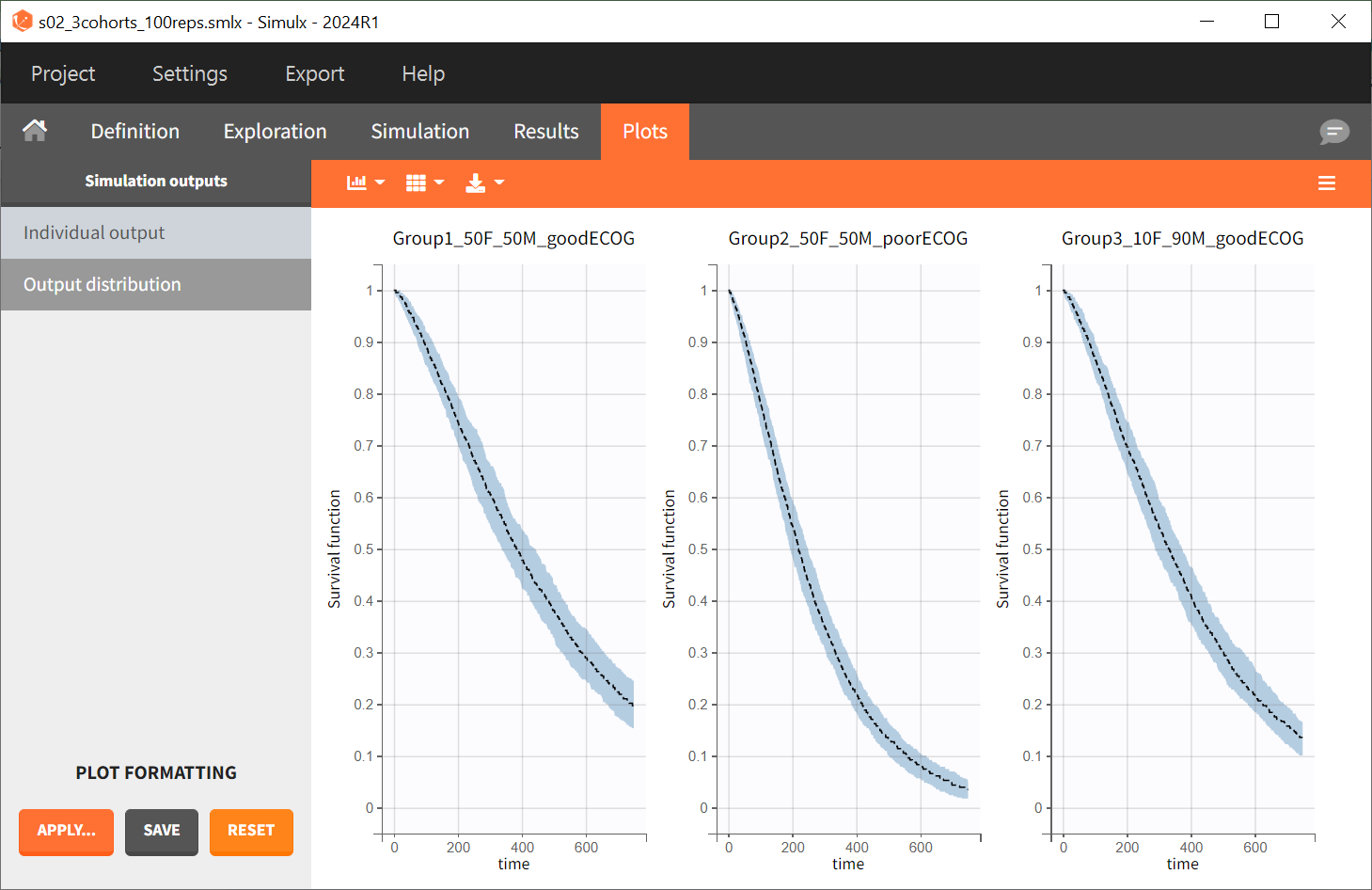
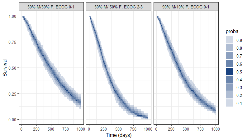
Since the time of death is a random variable, multiple simulations of the same population will result in different survival curves. To evaluate the uncertainty around the survival curve, replicates are generated by switching the simulation mode from "Single simulation" to "Replicates" in the scenario definition, with the number of replicates set to 100. The outputs now represent the prediction interval for the Kaplan-Meier curve.

To quantitatively compare the median survival, the post-processing tool in Simulx, called "Outcomes & Endpoints," is used. It calculates how many individuals survive for a specific duration and assesses the uncertainty of this result when simulating replicates. For instance, an outcome can be created to determine if an individual “has no event” between the observation's start (time = 0) and the end (time = 750).

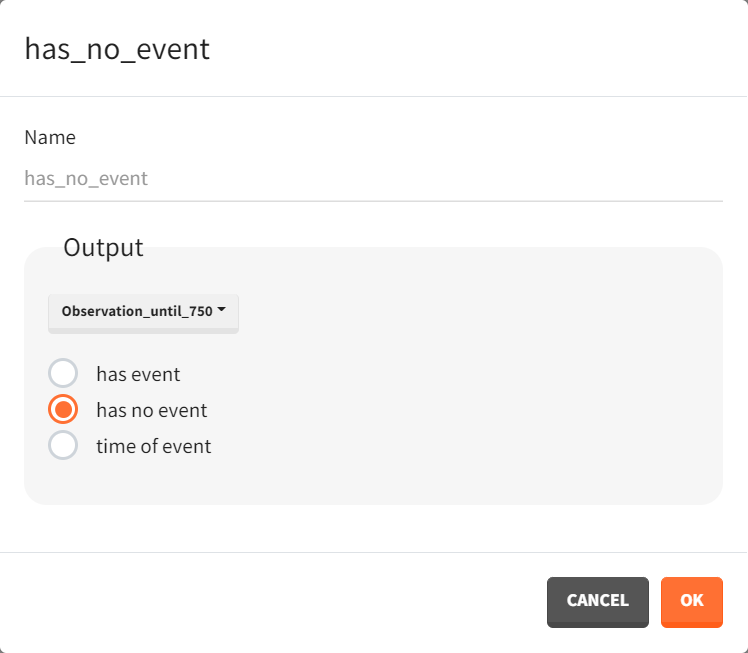
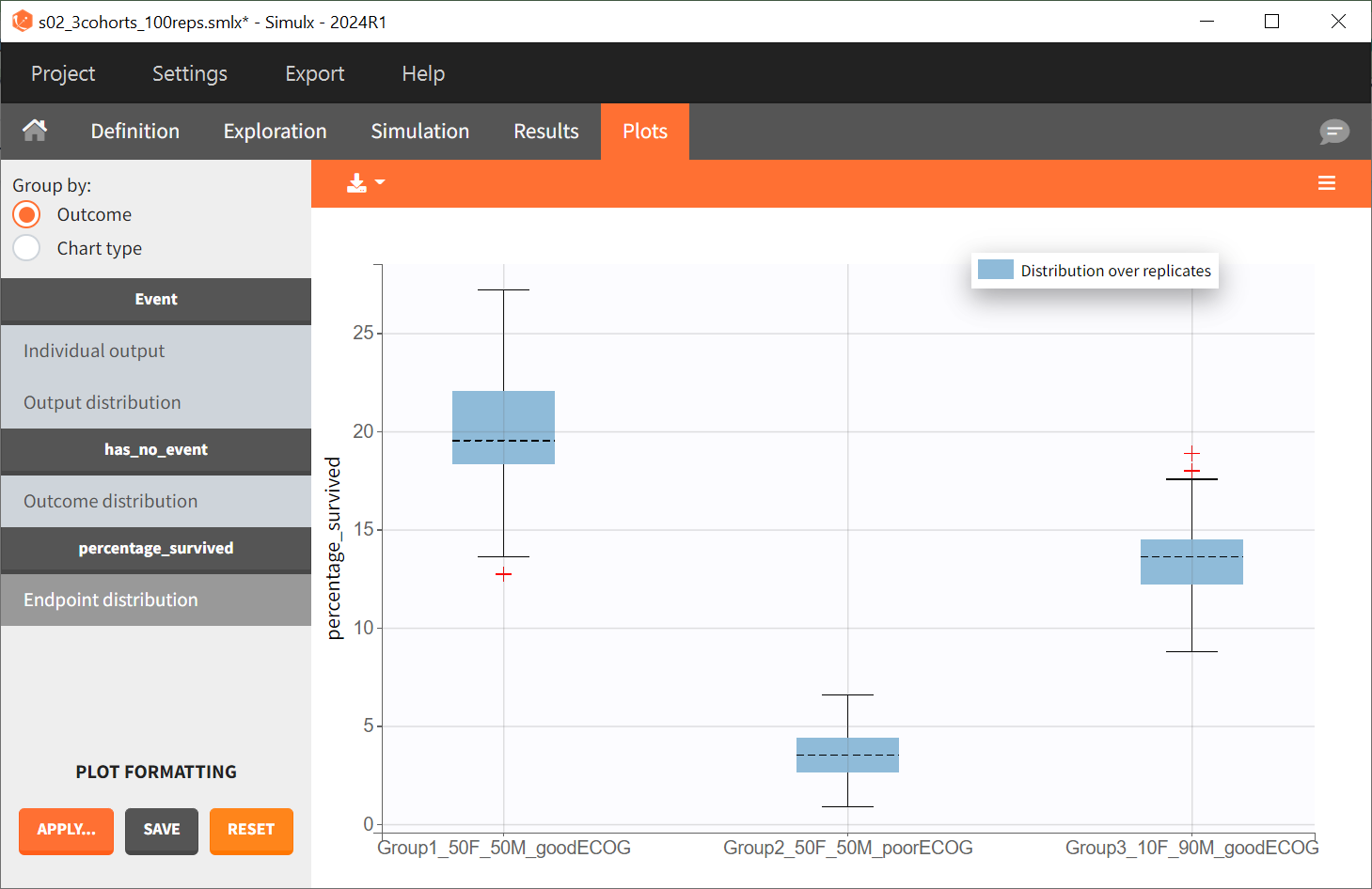
Then, this outcome is used in the definition of an endpoint: percent true

The results are presented in the results tables and as a boxplot in the plots tab:

The simulations performed in Simulx can also be conducted in R using either the RsSimulx package or the lixoftConnectors package.

Simulations via scripting with RsSimulx

The documentation on the RsSimulx R-function can be found here.

The same approach used in the previous section "Simulations using Simulx GUI" is applied here for simulating three new cohorts with different covariates:

cohort 1: 50% male / 50% female, good ECOG scores (0 or 1)
cohort 2: 90% male / 10% female, good ECOG score (0 and 1)
cohort 3: 50% male / 50% female, poorer ECOG scores (2 or 3)

The three groups are created via a data frame defining individual covariates, which are then passed as input to the simulx() function. This function returns an R object with the simulation results (time of death for each individual). These results can then be visualized with the kmplotmlx function, producing Kaplan-Meier survival curves.

For cohort 1, the corresponding R code reads as follows:

CODE

#========== defining group 1
# covariate data frame for group 1, with column id and one column per covariate
cov1 <- data.frame(id=1:228,
                   sex     = c(rep("F",114),rep("M",114)),
                   ecogPH  = rbinom(n=228, size=1, prob=0.5), 
                   karnoPH = rnorm(228,mean=80,sd=12.3),      #unused in model but must be present
                   karnoPAT= rnorm(228,mean=80,sd=14.5),      #unused in model but must be present
                   age     = rnorm(228,mean=63,sd=9))         #unused in model but must be present
          
#============= calling simulx for group 1
res1 <- simulx(project  = project.file,
               covariate= cov1)

The output objects are combined into one and plotted using the following command:

CODE

#============= plotting the KM survival curve
group.labels <- c("50% M/50% F, ECOG 0-1", "50% M/ 50% F, ECOG 2-3","90% M/10% F, ECOG 0-1" )
km <- kmplotmlx(EvRes,labels=group.labels,facet=FALSE) + 
  xlab("Time (days)") + 
  ylab("Survival") + 
  theme(legend.position = "bottom")

The prediction is as follows:

Since the time of death is a random variable, multiple simulations of the same population will result in different survival curves. The uncertainty of the survival curve can be assessed by performing replicates, which can be easily achieved by including the argument nrep.

CODE

res1 <- simulx(project  = project.file,
               covariate= cov1,
               group    = list(size=50),
               nrep     = 100)

A prediction interval for the three survival curves is then obtained:

Conclusion

The MonolixSuite is a powerful tool for modeling and simulating time-to-event data via a parametric approach. Covariates, frailty models, and censoring can easily be incorporated. Built-in statistical tests and diagnostic plots (in particular, the “visual predictive check for TTE data”) render the model development process straightforward.

With the lung cancer data set of this case study, the risk of death increases over time (Weibull distribution of death times). Sex and the ECOG performance score are significant covariates and thus prognostic factors. Performance scores assessed by patients rather than physicians can also serve as prognostic factors, but their utility in addition to the physician-measured score is minimal.

Thanks to the parametric formulation of the model, survival probabilities depending on sex and ECOG score can easily be computed. Additionally, simulations of cohorts with combinations of covariates can be performed using Simulx, and the uncertainty of the resulting survival curve can be visualized.