Modeling the pharmacokinetics and pharmacodynamics of warfarin in healthy volunteers

Download data set only | Download all Monolix project files | Download Simulx project files | Download Simulx R scripts

• Introduction and outline

• Data exploration and visualization

• Pharmacokinetic (PK) modeling

  • Examining PK data and initial trends

  • Structural PK model development

  • Assessment of parameter estimate robustness

  • Statistical PK model development

• Pharmacokinetic - Pharmacodynamic (PKPD) modeling

  • Examining PKPD data

  • Structural PD model development

• Simulations

  • Simulations scripted with lixoftConnectors

• Discussions and conclusions

Introduction and case study outline

O’Reilly (1968). Studies on coumarin anticoagulant drugs. Initiation of warfarin therapy without a loading dose. Circulation 1968, 38:169-177.

Warfarin is an anticoagulant normally used in the prevention of thrombosis and thromboembolism, the formation of blood clots in the blood vessels and their migration elsewhere in the body, respectively. The data set provides set of plasma warfarin concentrations and Prothrombin Complex Response in thirty normal subjects after a single loading dose. A single large loading dose of warfarin sodium, 1.5 mg/kg of body weight, was administered orally to all subjects. Measurements were made each 12 or 24h.

Case study outline

The case study begins with data exploration and visualization within Monolix. This exploration highlights key characteristics of the dataset, such as individual variability in plasma concentrations and the observed pharmacodynamic response over time.

In the section "Pharmacokinetic (PK) Modeling," the goal is to develop a robust PK model that accurately captures the observed data. The modeling process involves examining diagnostic plots, comparing different structural models, and refining the model using statistical tests and convergence assessments. Sycomore is employed for systematic model comparisons, enabling the selection of the most appropriate PK model.

The section "Pharmacokinetic-Pharmacodynamic (PKPD) Modeling" focuses on linking the pharmacokinetics to the observed pharmacodynamic response. Guided by visualization tools and prior knowledge, the model is developed iteratively, emphasizing the refinement of the pharmacodynamic component while maintaining consistency with the final PK model. Diagnostic tools, such as statistical tests and diagnostic plots, are used extensively to ensure the accuracy and reliability of the PKPD model.

The final section outlines the modeling workflow and demonstrates how the established PKPD model can be further validated and applied in simulations. The simulations will compare two treatment regimens by defining dosing schedules, outcome criteria, and statistical evaluation methods. Replicated simulations will be conducted to account for population parameter uncertainty, and the proportion of subjects meeting the efficacy criterion will be assessed. A statistical test will be used to evaluate statistical differences between groups, providing insights into the expected trial outcome.

Data exploration and visualization

The dataset originates from a clinical trial studying Warfarin, an anticoagulant commonly used to prevent thrombosis and thromboembolism—conditions involving the formation and migration of blood clots in the blood vessels.

Clinical trial details:

• Participants: 32 healthy volunteers.

• Administration type: Oral administration.

• Dosing regimen: A single large loading dose of Warfarin sodium was administered. The dose was calculated as 1.5 mg/kg of body weight for each subject.

• Measurement schedule: Plasma concentrations and Prothrombin Complex Activity (PCA) were measured at time intervals of 12 or 24 hours post-dosing.

Pharmacokinetic (PK) and pharmacodynamic (PD) data:

• PK: Warfarin concentrations in plasma.

• PD: Prothrombin Complex Activity (PCA), which reflects Warfarin's pharmacodynamic effect.

The columns in the dataset are:

• id: The subject ID, column-type ID.

• time: The time of the measurement or dose, column-type TIME.

• amt: The amount of drug administered to each subject, column-type AMOUNT (1.5 mg/kg of body weight, consistent across all subjects).

• dv: The dependent variable (measured values), column-type OBSERVATION.

  • For PK data: Plasma concentrations of Warfarin.

  • For PD data: Prothrombin Complex Activity (PCA).

• dvid: The type of measurement:

  • DVID = 1 corresponds to PK measurements (Warfarin concentrations).

  • DVID = 2 corresponds to PD measurements (PCA).

• wt: Subject weight (kg), column-type COVARIATE.

• sex: Subject sex (0 = female, 1 = male), column-type COVARIATE.

• age: Subject age (years), column-type COVARIATE.

Pharmacokinetic (PK) modeling

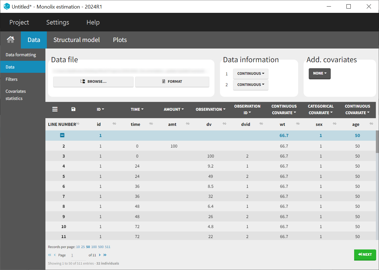
After a new project has been created, the data uploaded, and the columns correctly tagged, the observations can be visualized in the observed data plot.

Examining PK data and initial trends

It quickly becomes apparent that some profiles have no or only very sparse absorption phases. This could later impact the estimates of the absorption parameters, as there is simply less information available about the early phase of the profiles.

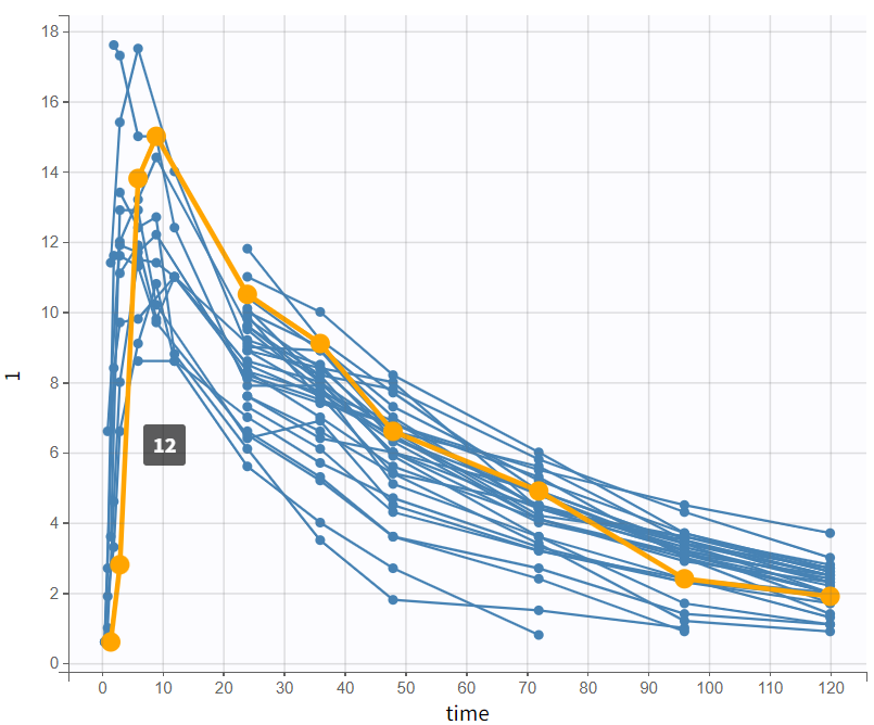
By log-scaling the y-axis, a first impression of the elimination phase can be obtained. This allows for identifying whether it follows a linear (positive curvature) or non-linear pattern (negative curvature), and whether it can be described by a single slope or multiple linear segments. This helps determine the number of compartments to consider and choose:

The majority of subjects exhibit a profile with a simple slope in the elimination phase, suggesting that a one-compartment model with linear elimination is a good choice for the initial structural model.

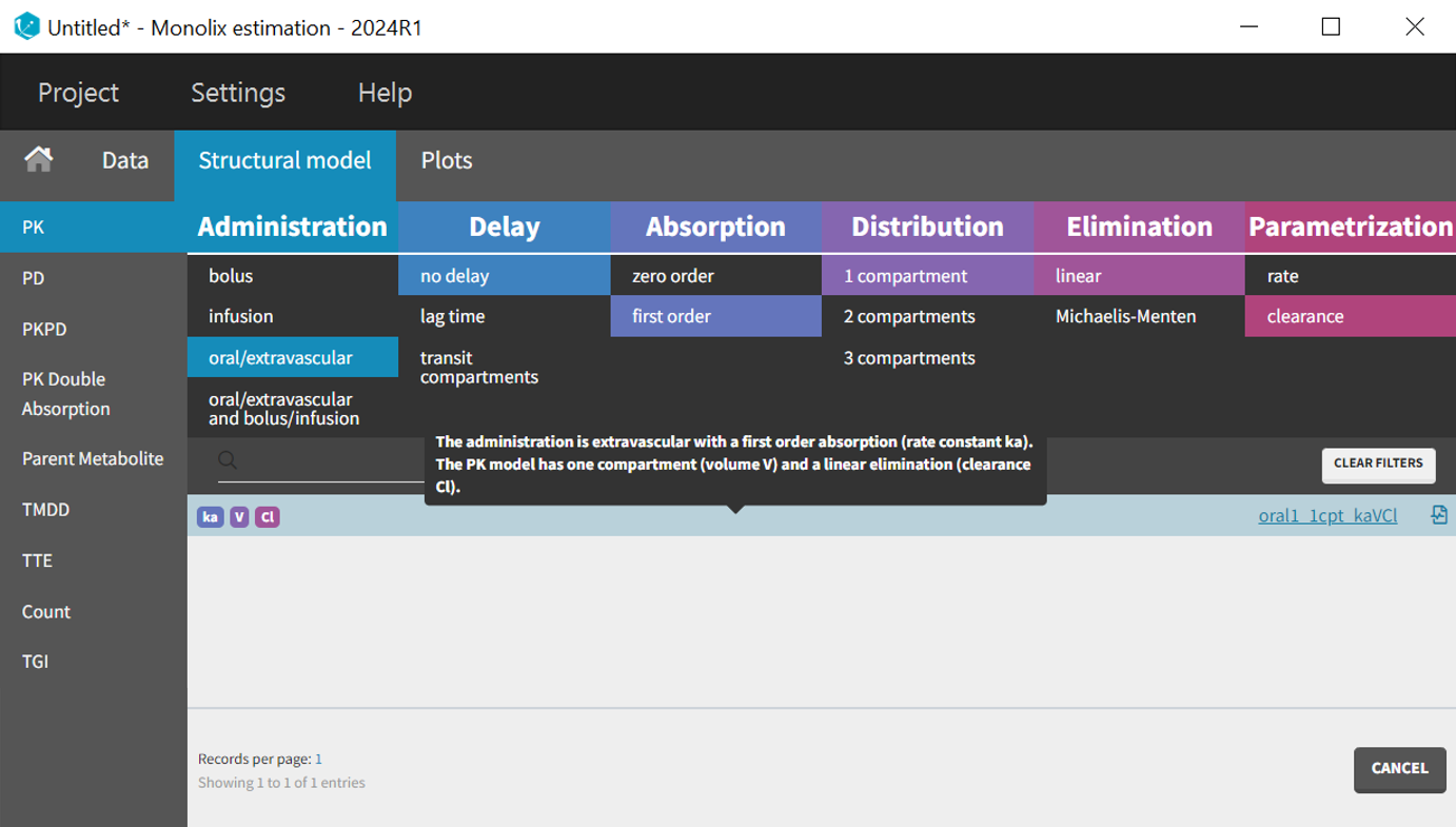
Structural PK model development

In the model library of the PK model class, various filters can be applied that relate to different phases of the time profiles. The treatment administration regime indicates that the drug was administered orally, and no delay in the absorption phase was observed in the data. First order absorption is selected, as most drugs exhibit first-order absorption. A one-compartment model seems to be a good starting point, with linear elimination and clearance (Cl) parameterization (lib:oral1_1cpt_kaVCl.txt). Finally, the choice of parameterization (ke or Cl) is not crucial, as they are equivalent.

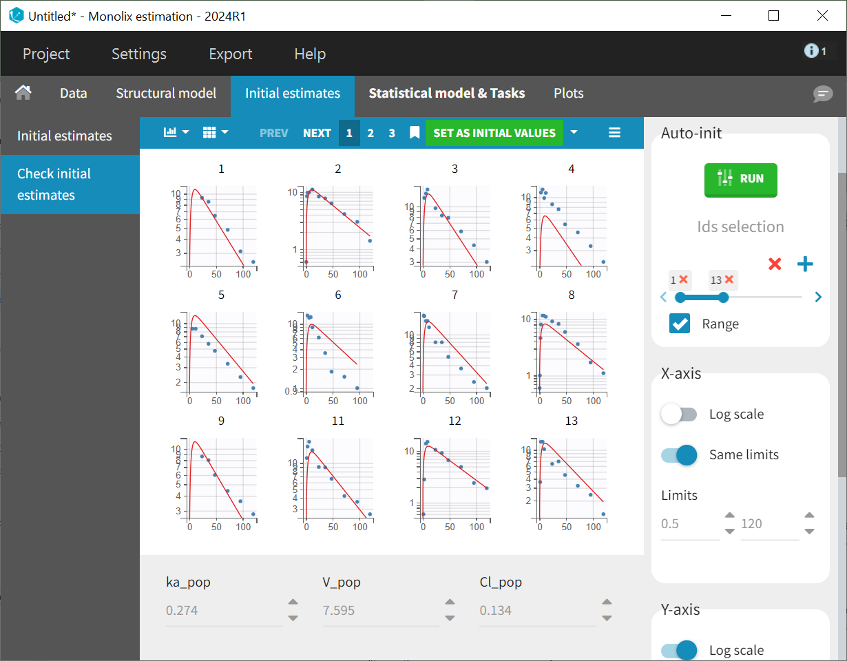
After selecting the one-compartment model, the "Initial estimates" tab is used to define initial values for the three population parameters. The auto-init function was used to automatically propose reasonable starting values. These initial values should capture the main characteristics of the profiles. This process focuses on the typical profile shape and does not account for inter-individual variability. The log scale applied to the Y-axis helps confirm that the elimination phase is well captured by the one-compartment model.

The initial values are applied to the estimation tasks by clicking the green "Select as initial values" button, which redirects to the "Statistical model & tasks" tab. This tab lists the individual estimation tasks and includes the observation model, which links observations and predictions by incorporating an error term. The statistical model can be further refined in the individual model section. At this stage of modeling, the focus is on establishing a well-fitting structural model before adjusting the statistical model. Therefore, the default settings for the observation and individual models are maintained, with adjustments to be evaluated later as needed.

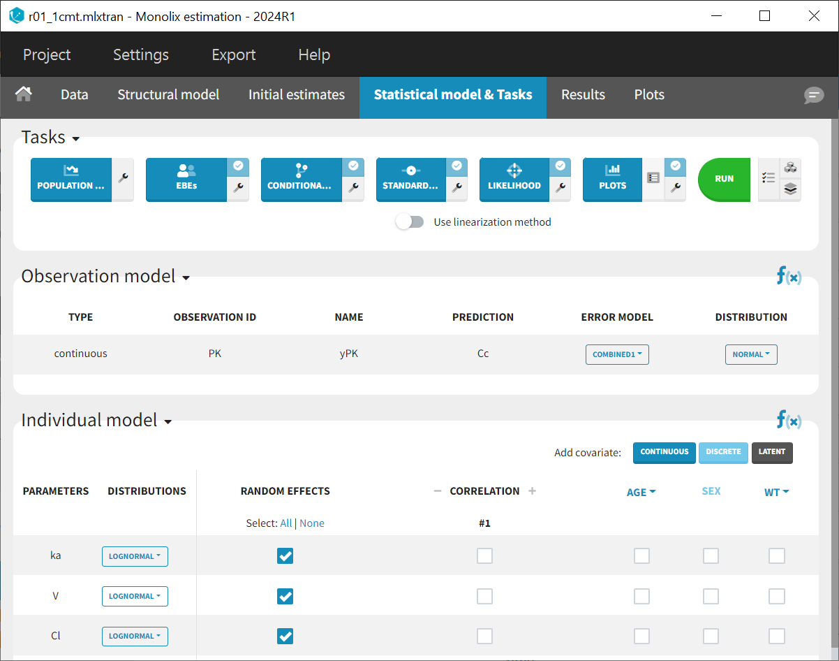
This model comprises a combined residual error model with both additive and proportional terms, log-normal distributions for the three parameters and along with random effects on all parameters and . Correlations between random effects and covariate effects on parameters are not included at this stage. All elements are set to their default configurations, ensuring that the tasks listed in the top panel of the "Statistical model and tasks" tab are ready to be launched.

Tasks are executed to estimate the parameters and assess the model fit to the data. Before running any tasks, it is recommended to save the project (Menu > Save as> r01_1cmt.mlxtran) to ensure that all result text files generated during the tasks are stored in a folder alongside the project file.

The “Population parameters” and “EBEs” tasks estimate both population and individual parameters. The “Conditional Distribution” task enhances diagnostic plots and the conduct of statistical tests, particularly with small sample sizes. The “Standard error” task estimates the standard error and relative standard error of the population parameters, while the “Likelihood” task calculates the objective function to identify the best population parameters. The “Plots” task is included for model diagnostics. The scenario is executed by clicking the green 'Run' button.

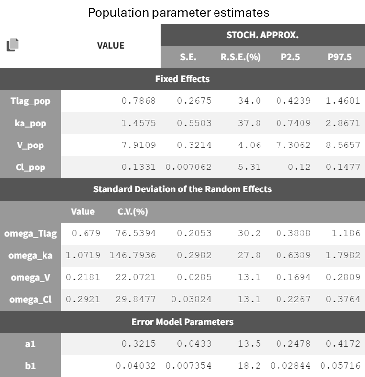
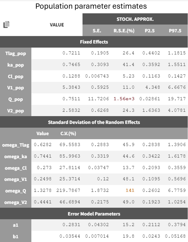
After running the estimation tasks, a "Results" tab becomes available, where additional plots in the "Plots" tab assist with model evaluation. Below is the results table from the "Results > Pop. param" tab.

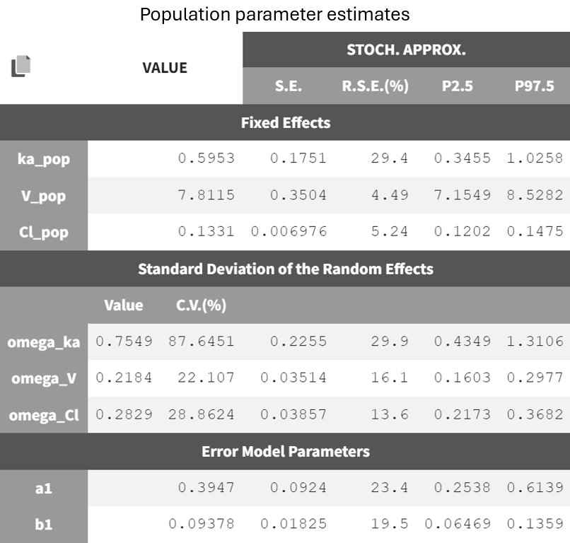
It displays the estimates of the population parameters for fixed effects and as well as the standard deviation of the corresponding random effects (all parameters). Each parameter also has standard error estimates, relative standard error estimates, and confidence interval limits. The parameters appear to be estimated with good certainty.

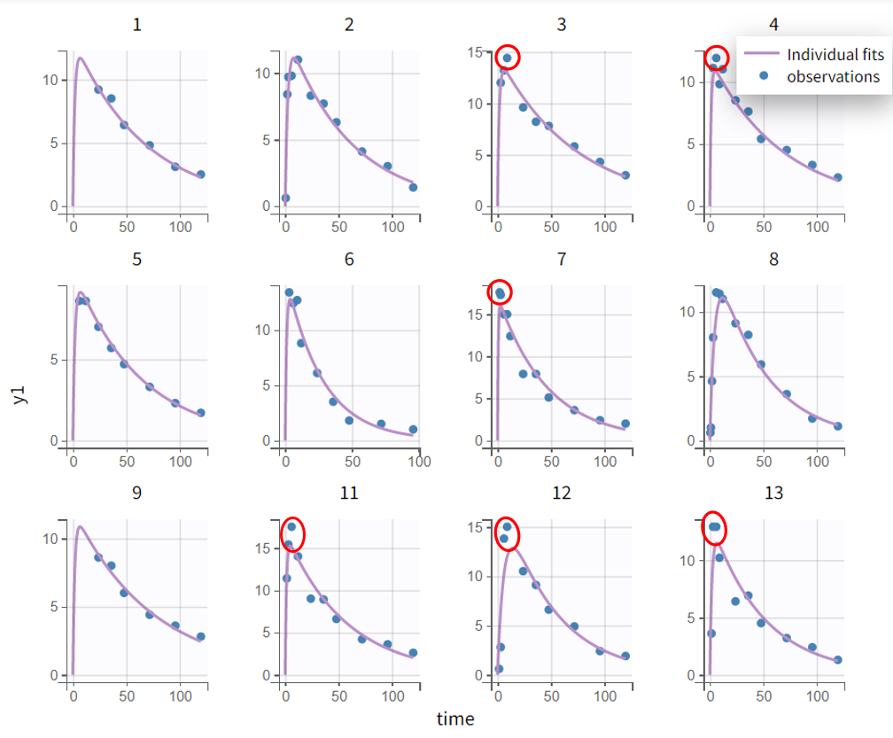
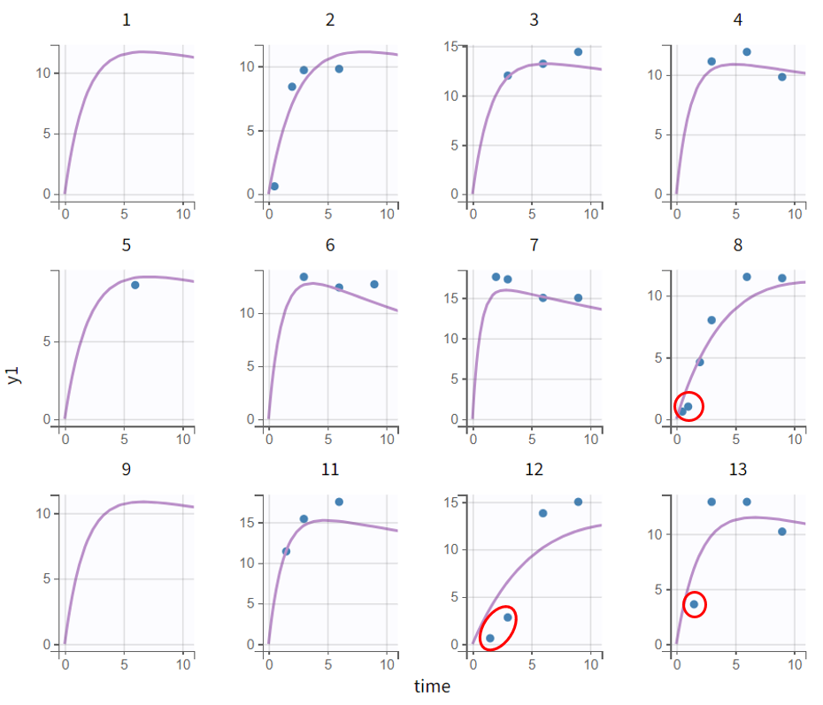
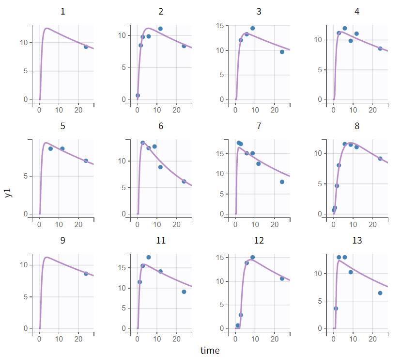
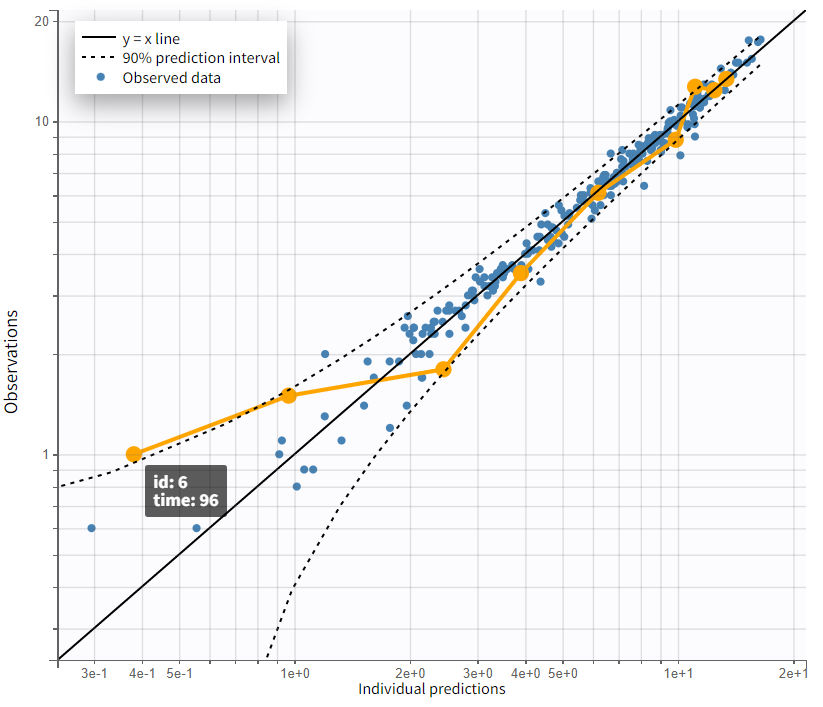
In the individual fits plot in the "Plots" tab, the prediction curve based on individual parameters (here, by default EBEs) is shown alongside the observed data. It is apparent that the peaks (the highest measurements) are under-predicted for many subjects. Zooming in on the early phase (the absorption phase) for all subjects (Zoom constrain x-axis > Link zoom between plots) reveals that the first data points in profiles with early measurements are over-predicted.

Complete profile	Early absorption phase (zoomed-in)

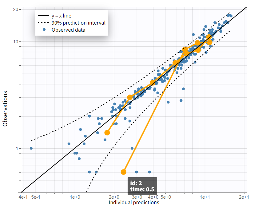
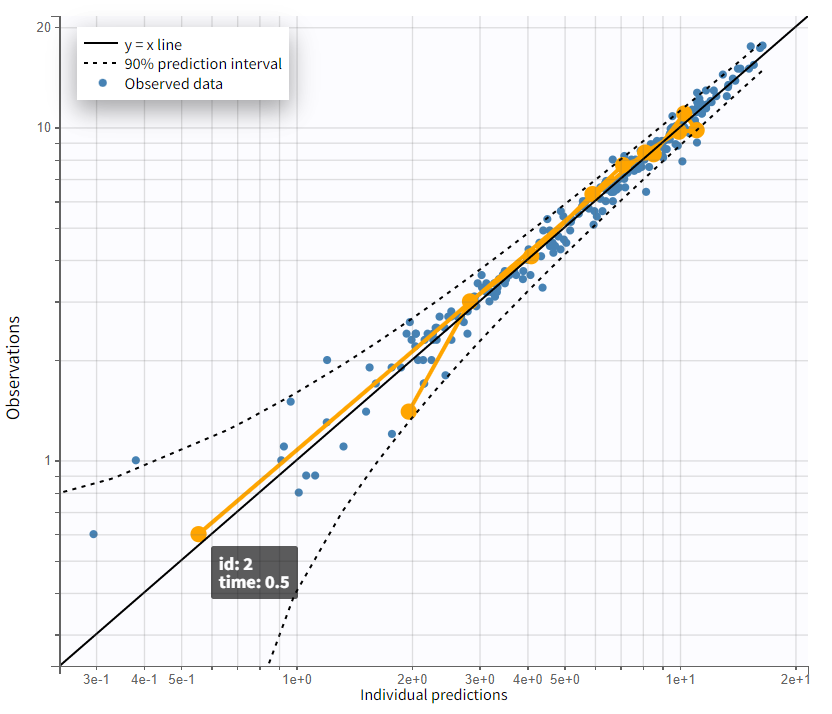
The evaluation of the individual fits plot suggests that adding a lag time to the model could be beneficial. This is further confirmed by the observation vs. prediction plot. After log-log scaling the plot, the data from early time points are significantly below the identity line, indicating they are over-predicted.

The next modeling step should be to include lag time. This would cause the prediction curve to rise later but steeper, better capturing the early and highest measurements.

To accelerate convergence for the next model run, population estimates can be used as initial values by selecting "Use last estimates: Fixed effects" in the "All" in the "Initial estimates" tab. Then, in the "Structural model" tab, the delayed first-order absorption model (lib:oral1_1cpt_TlagkaVCl.txt) is selected by changing the filter from “no delay” to “lag time”.

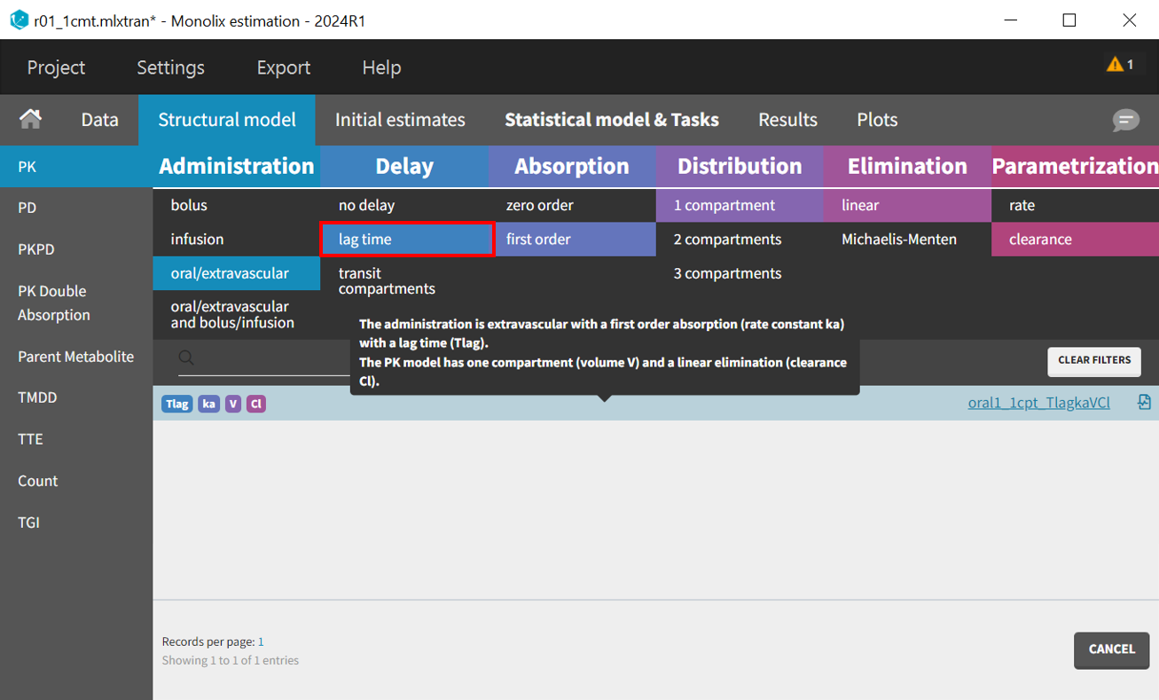
In the "Initial estimates" tab, an appropriate initial value for Tlag_pop should be set, typically between 0 and 1.5 based on the individual fits and observations vs predictions plot, with 0.5 being a reasonable selection. The initial values for the other five parameters remain as previously estimated.

The updated project can be saved as r02_Tlag_1cmp_Tlag.mlxtran, and the same scenario can be executed.

The estimates for and remain close to the previous values, while and increased. This is coherent with the model adjustments, which only affected the absorption phase. The estimates remain within a range that can be considered reliable and certain. By evaluating the diagnostic plots below, it is clear that adding a lag time was beneficial.

Individual fits - early absorption phase (zoomed-in)	Observations vs. predictions

Focusing on the elimination phase of the time profiles, it is visible for a few individuals, such as 6, 7, and 11, that an additional slope would better capture the final data points. This would suggest the inclusion of a second compartment. The observation vs. prediction plot also confirms that points further from the identity line correspond to later observations. However, this observation applies only to a few individuals.

Complete profile - semi log scaled	Observations vs. predictions

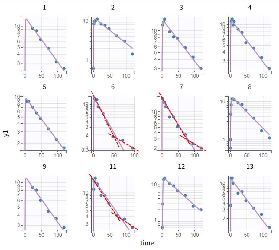
The next step in model development involves the inclusion of a second compartment. Before changing the structural model, selecting "Use last estimates: All" ensures that the final estimates from the current run, which were determined with good confidence, are used as initial values for the next run. This provides a strong starting point for SAEM, aiding the convergence. The structural model is then adjusted by changing the filter in the PK model library under "Distribution" from one compartment to two compartments. Initial values for the new parameters and are determined either manually or using the auto-init function, which identifies the best overall fit. The initial values are set as follows: and . The omega parameters of the unchanged parameters retain the values from the previous run, while the omega parameters of the new ones are initialized with a value of 1. The project is saved under a new name (r03_Tlag_2cmt.mlxtran), and the scenario is executed.

In the results tab for population parameters, the estimation of shows very high uncertainty, affecting both the fixed effect and the standard deviation of the random effect . This indicates that the parameter is difficult to estimate, which aligns with observations from the diagnostic plots. Only a few individuals exhibit characteristics of a second compartment, resulting in limited contributions to the SAEM algorithm for reliably estimating parameters related to the second compartment.

The plots overall demonstrate a good fit.

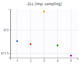
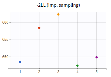
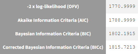
To enable a quantitative comparison between models during the model development process, the Monolix project can be exported to Sycomore. This is done via the export menu: Export > Export project to ... > Target software: Sycomore. Sycomore facilitates the calculation and visualization of metrics such as BICc, qnd -2LL, allowing for a robust comparison of model performance.

What can be stated with certainty is that the inclusion of a lag time in the absorption profile led to a significantly improved fit. The difference in -2LL and BICc between run 2 (r02_Tlag_1cmt.mlxtran) and run 1 (r01_1cmt.mlxtran) amounts to and .
The likelihood estimate also improved in the two-compartment model (r03_Tlag_2cmt.mlxtran) compared to the one-compartment model (r02_Tlag_1cmt.mlxtran), reflecting a better fit to the data. However, the BICc did not improve in the same magnitude, indicating that the increase in model complexity might not be justified statistically.

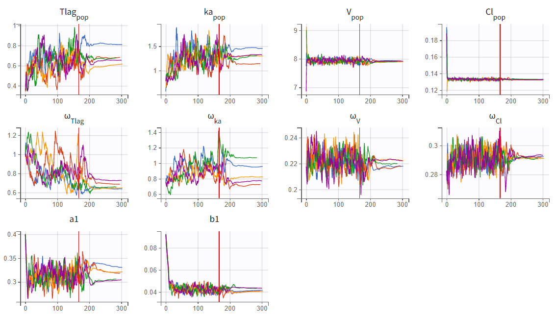
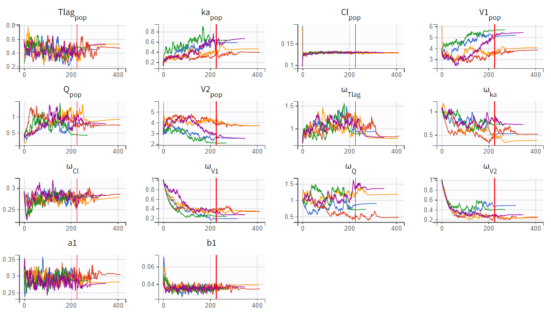
Assessment of parameter estimate robustness

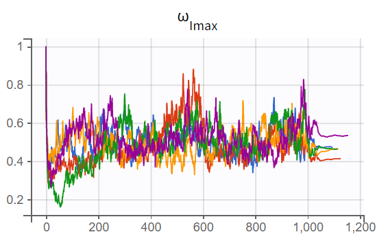
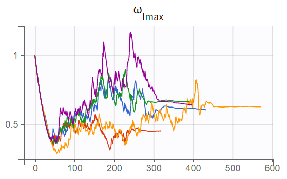
To assess the stability of parameter estimates, the convergence assessment was performed by running the scenario five times with different seeds and slightly varied initial values. For the two-compartment model (r03_Tlag_2cmt.mlxtran), the parameter and likelihood estimates showed significant variability across runs, indicating unstable convergence. In contrast, the one-compartment model (r02_Tlag_1cmp.mlxtran) demonstrated stable and consistent estimates.

1-compartment model with Tlag (r02_Tlag_1cmp.mlxtran)	2-compartment model with Tlag (r03_Tlag_2cmt.mlxtran)

In the convergence assessment, the trajectories for ​ and in both runs diverge, likely due to some subjects lacking measurements in the absorption phase. While all subjects have measurements in the elimination phase, the SAEM trajectories for parameters related to the second compartment in run r03_Tlag_2cmt.mlxtran also show divergence. This is because only a few subjects display characteristics of a second compartment in their profiles. As a result, the estimates in r03_Tlag_2cmt.mlxtran are less stable and more uncertain, which is also reflected in the high uncertainty of the parameter. Overall, model r02_Tlag_1cmp.mlxtran provides a good fit while ensuring more robust and reliable parameter estimates, making it the preferred final structural model.

Statistical PK model development

Adjustment to the residual error model

Model development begins by evaluating the structural model to ensure it captures the key profile characteristics, followed by selecting the best error model to account for prediction-observation deviations.

The selection of the residual error model is guided by the Results tab "Proposal," where different error models (constant, proportional, combined1, combined2) are evaluated. The criterion is calculated for each error model, with the error parameters optimized based on the data and the predictions generated by the final structural model.

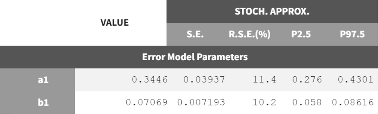
The combined2 error model appears to fit the data better than the combined1 error model. Unlike combined1, which assumes a linear relationship between error and prediction, combined2 accounts for nonlinearity by modeling the total error as the square root of the sum of squared constant and proportional terms.

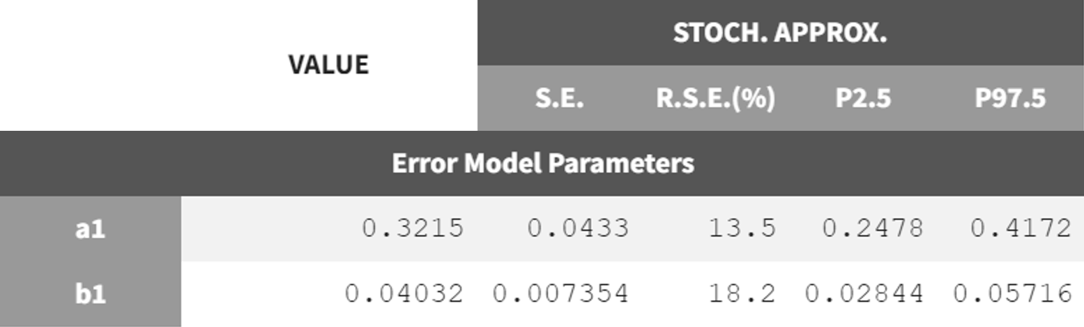
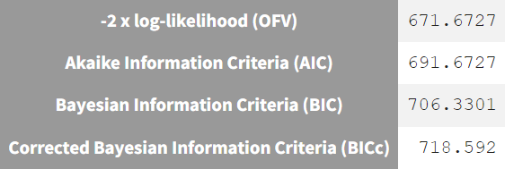
The next step is to switch to the combined2 error model. The final estimates from r02_Tlag_1cmt.mlxtran are used as initial values, the project is saved under a new name (r02_1_Tlag_1cmt_comberr2.mlxtran), and the estimation tasks are launched. The error parameters and remain in the same range as the previous estimates but show lower RSE values. Additionally, the information criteria indicate that switching to the combined2 error model has improved the model fit.

r02_Tlag_1cmp.mlxtran - combined 1	r02_1_Tlag_1cmt_comberr2.mlxtran - combined 2

Covariate model

After establishing the base model, the next step is to incorporate covariate effects that influence the distribution of individual parameters. If these effects are not included, their contribution to variability remains within the variability of the random effects.

The dataset contains only a few covariates, allowing for a manual forward inclusion and backward elimination approach to develop the covariate model. Each model run includes the conditional distribution and plots tasks, generating statistical tests and diagnostic plots to identify influential effects.

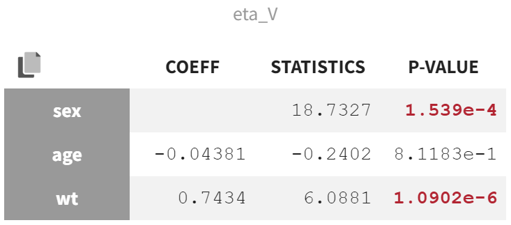
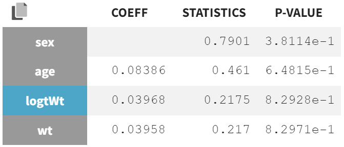
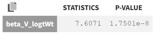
In the "Test" section of the Results tab, the random effect shows the strongest covariate effects. The lowest p-value is from the correlation test between body weight (wt) and , assessing whether the correlation coefficient differs significantly from zero.

The second-lowest p-value comes from the ANOVA Type III test, which evaluates the effect of sex on . A significant p-value in this test indicates that the variance in is significantly different between the two sex modalities. This suggests that the mean values of for males and females are significantly distinct, and the variability in is not the same for both groups.

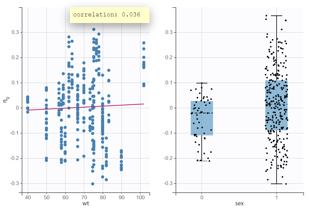
The "Individual Parameters vs Covariates" plot confirms these findings. The scatterplot of vs. wt shows a steep regression line, while the boxplots of grouped by sex modality reveal a clear separation in both mean and spread.

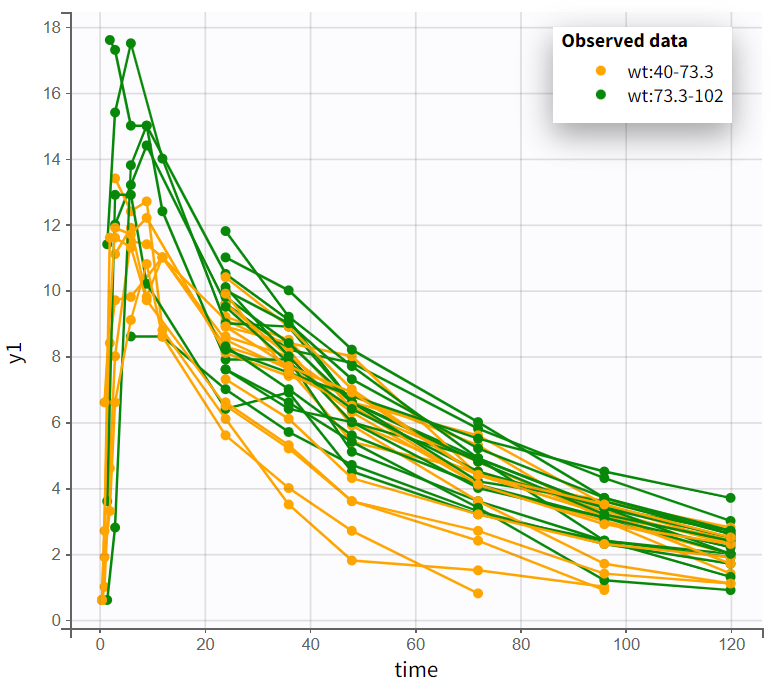
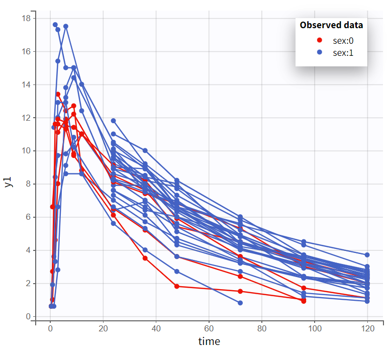
In the “Observed data” plot, coloring profiles by weight shows that subjects with higher body weight tend to have higher concentrations, even though the drug was administered weight-normalized. Coloring by sex shows that male subjects tend to have higher concentrations than female subjects.

Observed data plot - colored by weight	Observed data plot - colored by sex

In the manual forward inclusion and backward elimination approach, the strongest effect is first considered, which in this case is body weight wt on volume . The covariate is included via a power law relationship. To transition from the lognormal domain to the gaussian domain, the covariate must be log-transformed.

In Monolix, selecting a continuous covariate in the individual model prompts a suggested log transformation (“Add log-transformed“), creating a new column where the covariate is logarithmized and normalized by a typical population value.

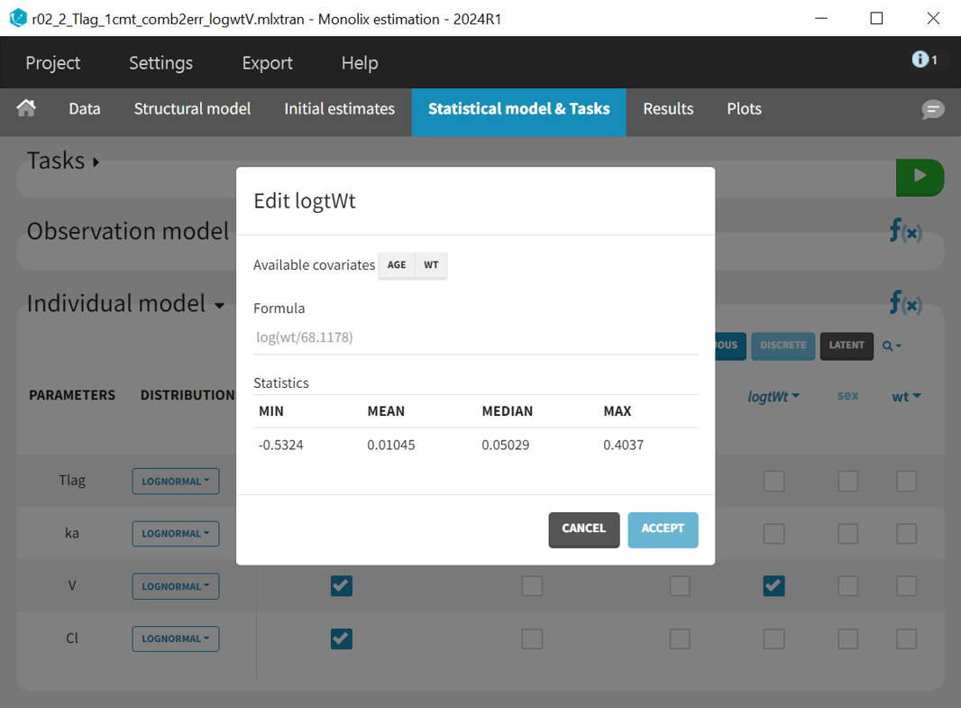
The new covariate logWt is added to the individual model for parameter . The last estimates are used as initial values, the project is saved under a new name (r02_2_Tlag_1cmt_comb2err_logwtV.mlxtran), and the estimation task is launched.

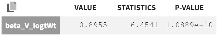
The new population parameter ​ appears in the population parameter table as a fixed effect, estimated with good certainty.

Forward inclusion	Backward elimination
Correlation test/ ANOVA	Wald test	Correlation test

Statistical tests show that wt and logWt no longer have significant p-values for ​, confirming their relevance in the forward inclusion step.

For backward elimination, additional tests are performed:

• Correlation test: Assesses if the regression coefficient between covariates and transformed parameters differs from zero.

• Wald test: Evaluates whether the estimated is significantly different from zero, using standard errors.

Both tests yield significant p-values, indicating that the effect is considered relevant and should remain in the model. Additionally, the inclusion of wt corrected the previously observed sex effect, indicating that the sex difference was likely due to wt-related variability distortions in .

In the plot “Individual parameters vs. covariates“ the accounted weight effect visibly corrected the distribution of ​, reducing distortion. The scatter plot of vs. wt now shows a less pronounced trend, and the boxplots grouped by sex reveal a reduced difference in mean and spread. The previously observed sex effect disappears when accounting for weight, likely because heavier subjects in the population are generally male, while lighter subjects are more often female. In other words, weight and sex were correlated.

Comparing information criteria of the current model run (r02_2_Tlag_1cmt_comb2err_logwtV.mlxtran) with the previous model without covariate effects (r02_1_Tlag_1cmt_comberr2.mlxtran) shows a likelihood difference of and a BICc difference of , confirming that capturing and explaining variability with WT was beneficial.

The stepwise forward inclusion and backward elimination of covariates continues until no significant effects remain.

The final model includes a weight effect (logtWt) on and , and an age effect (logtAge) on , leading to the lowest information criteria and . However, this model slightly inflates the RSE of . Backward elimination tests show borderline p-values, just below 0.05. Comparing the run with only logtWt on and (r02_3_Tlag_1cmt_comb2err_logwtVCl.mlxtran) to the final model with logtWt on and & logtAge on (r02_4_Tlag_1cmt_comb2err_logwtVCl_logageCl.mlxtran) shows a difference and , indicating only a minor improvement in variability explanation.

No significant correlations between random effects were detected, concluding the PK model development.

Pharmacokinetic - Pharmacodynamic (PKPD) modeling

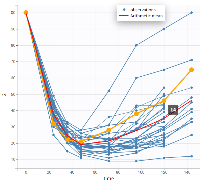
The next step is to describe the effect of warfarin on blood clotting. This is done by looking at prothrombin complex activity (PCA), which measures how well certain clotting factors in the blood are working.

Examining PKPD data

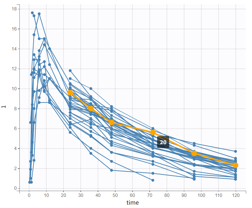
The PCA values range from 0 to 100. The spaghetti plot shows PCA starting at 100 at time 0, decreasing, and then gradually increasing again. PCA declines as PK concentrations rise, but not simultaneously—the lowest PCA values do not coincide with the highest PK values, indicating a delay.

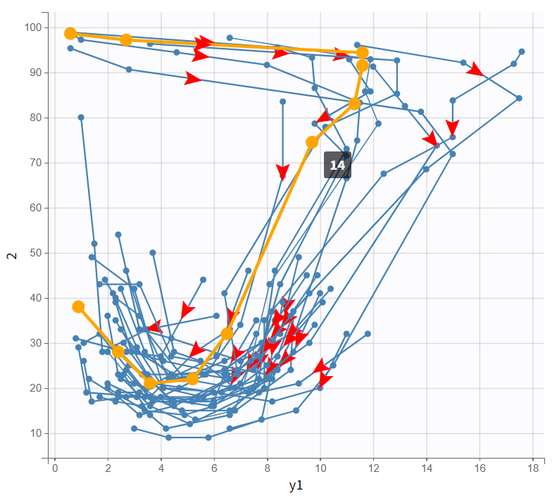
The bivariate plot confirms this pattern. With PK data on the x-axis and PD data on the y-axis, PD values remain relatively constant at first as PK increases. Then, a rapid drop occurs, forming a downward-curving loop. This behavior clearly rules out a direct PK-PD relationship.

Observed data plot	Bivariate data viewer

These PKPD relationship characteristics suggest two possible models, both describing how warfarin inhibits prothrombin complex activity (PCA): an effect compartment model or a turnover model.

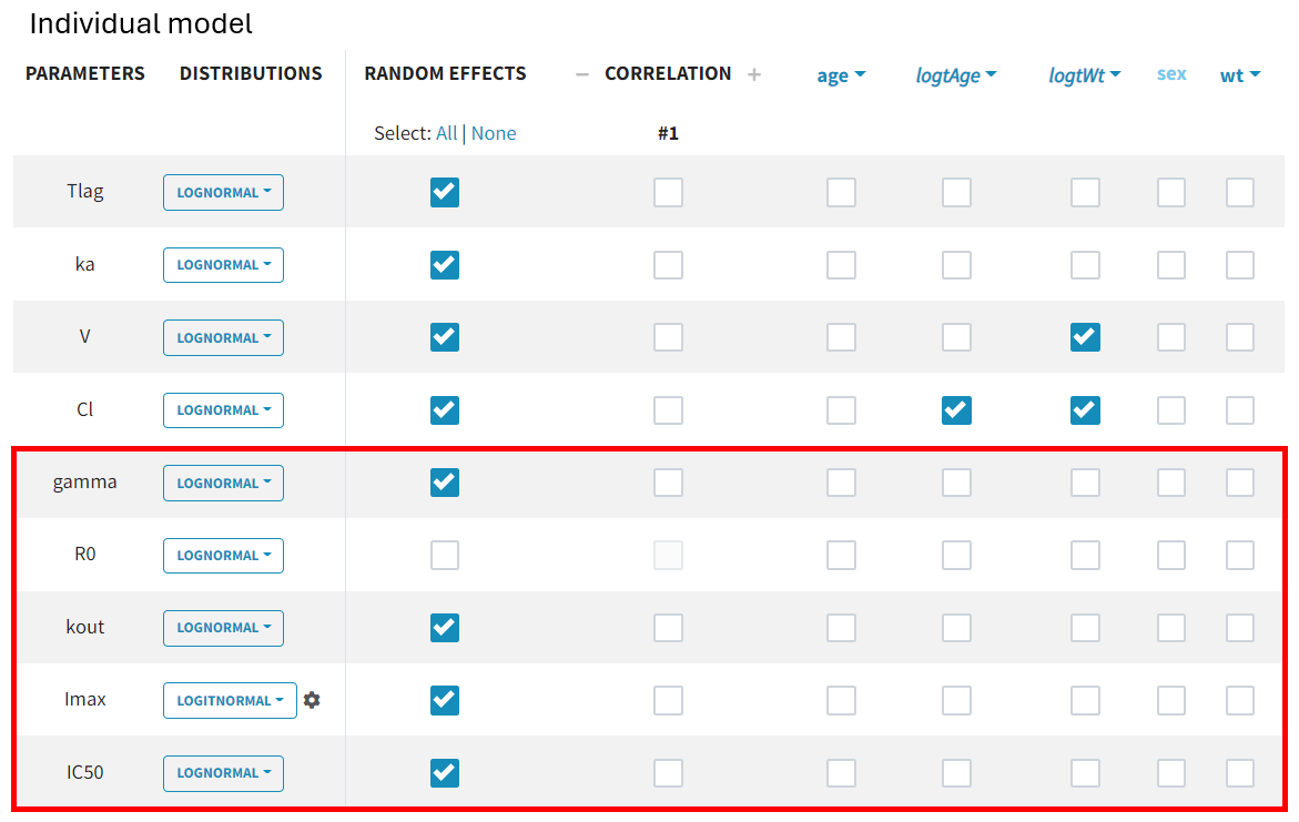
Structural PD model development

For modeling PD data, PK parameters should not be re-estimated, as reliable estimates are already available. In the “Initial Estimates” tab, selecting “Use last estimates: All” applies the previously estimated PK values. To keep them fixed, “Fix parameter values: All” is selected below.

In the “Structural Model” tab, the PKPD model class retains the filter for the PK model, requiring only the selection of the appropriate PD model. The turnover model is chosen with production inhibition as the drug action filter, specifically partial inhibition, since PCA values do not drop to zero. Sigmoidicity is also selected, introducing the variable , which adds flexibility by allowing a sigmoidal response curve. If is estimated close to 1, the model can still be simplified.

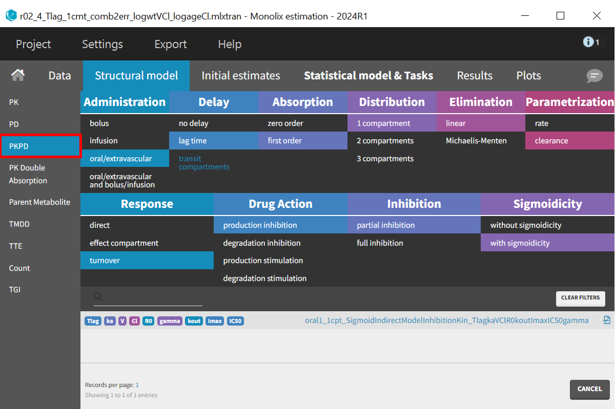
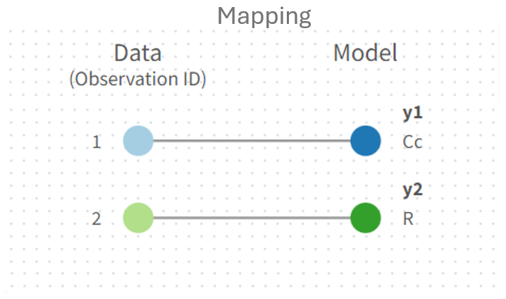
The prediction vector is mapped to observation id dvid= 2 in the panel next to the structural model.

In the “Initial estimates” tab, the parameter is set to 100 and fixed, as it corresponds to the baseline value of the PCA time profiles, with all subjects starting at 100. This ensures that , like the PK parameters, remains unchanged during the estimation tasks.

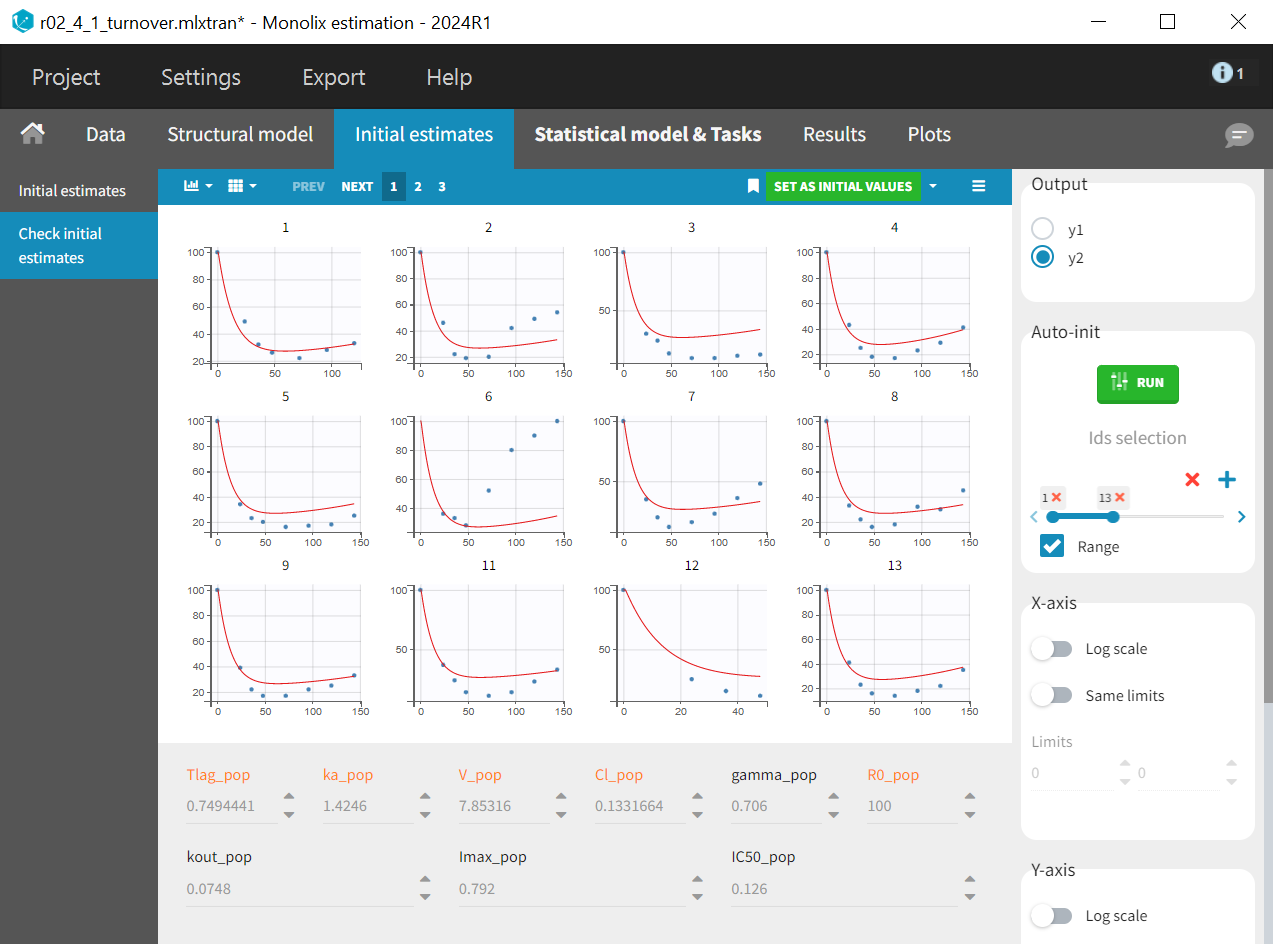
In the “Check initial estimates“ subtab the correct output radio button must first be selected to display the PD plots - in this case. Then the auto-init function is applied to find initial population parameters that best fit the data points for the PD data, while the PK parameters and , which appear in orange.

In the “Statistical model & task” tab, below the observation model , the PD observation model is now also displayed. It retains the default settings for the error model and distribution assumption.

Since PCA values range between 0 and 100 and follow therefore a logit-normal distribution, the distribution setting must be adjusted accordingly. To define the boundaries, the lower limit is set to 0, and the upper limit to 100.1, ensuring that 100 is included, as all subjects start from a baseline of 100. Additionally, the error model for the PD observations needs to be changed from the default combined1 to constant, as it is better suited for the logit-normal distribution of the PCA measurements

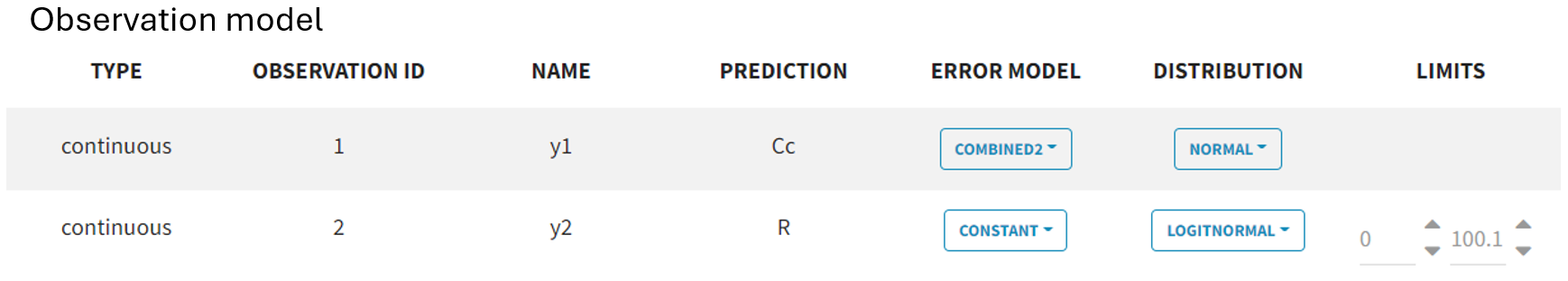
By default, all parameter distributions are set to lognormal, except for , which is logit-normal, as its values range between 0 and 1. Monolix applies this setting automatically when recognizing standard parameter names from the library. If an uncommon parameter name is used, Monolix defaults to a lognormal distribution. In such cases, the distribution must be adjusted before initializing estimates, as auto-init selects values based on the predefined distribution range.

Since the parameter corresponds to the baseline value of the PD data and is the same for all subjects, inter-individual variability is not considered. The random effect can therefore be removed.

No further model adjustments are required. The project can be saved under a new name (r02_4_1_turnover.mlxtran).

The turnover model has now been fully set up, covering all necessary steps from model selection to parameter initialization and error model adjustments. Another potential approach for describing the PKPD relationship is the effect compartment model. While structurally different, its implementation follows the exact same steps as the turnover model, with only differences in parameter names.

Turnover model	Effect compartment model

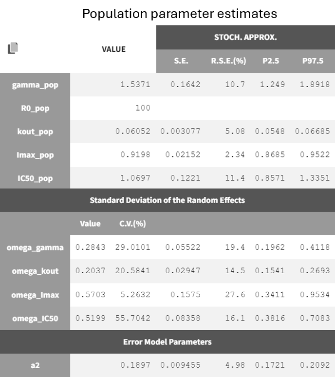
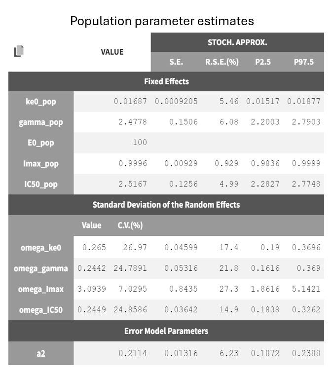
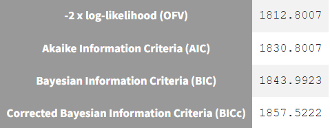
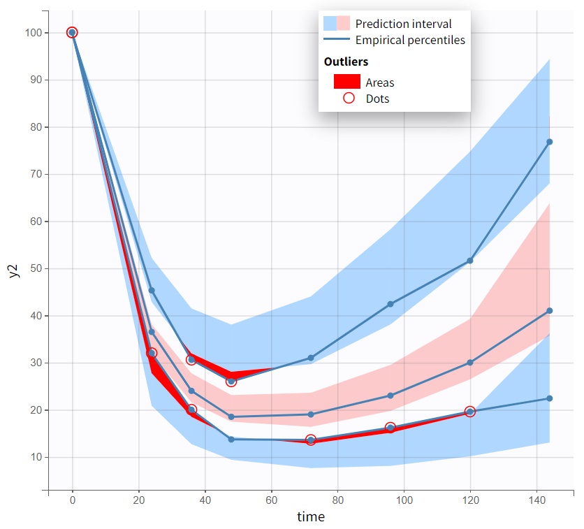
Both models yield similarly well-estimated population parameters with relatively good certainty. However, the effect compartment model has significantly higher BICc and -2LL compared to the turnover model. The VPC plot also indicates clear model misspecification in the effect compartment model, as the outer empirical percentiles (10th and 90th) systematically fall outside the theoretical percentiles during the decline of PCA. This suggests a misrepresentation of the delayed effect. In contrast, the VPC plot of the turnover model shows that the empirical percentiles mostly remain within the theoretical percentiles throughout the time profile.

Based on the evaluation of results and diagnostic plots, the turnover model better captures the PCA data and is selected as the final model.

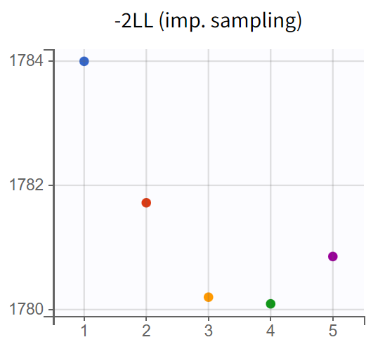
Assessment of parameter estimate robustness

At this stage, it is necessary to verify whether the final model also produces stable estimates by performing a convergence assessment, as done previously during the development of the PK model. Five runs are conducted with different initial values and different seeds. If the estimates are robust, the five final parameter estimates should be closely aligned, along with the log-likelihood values.

Convergence assessment (r02_4_1_turnover.mlxtran)
SAEM - Trajectories	-2LL

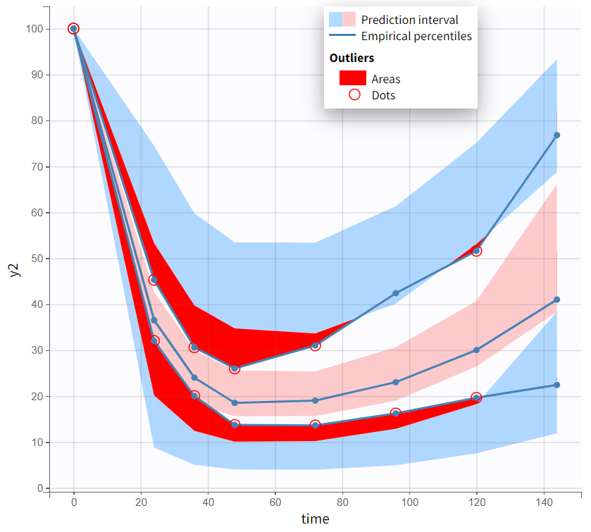
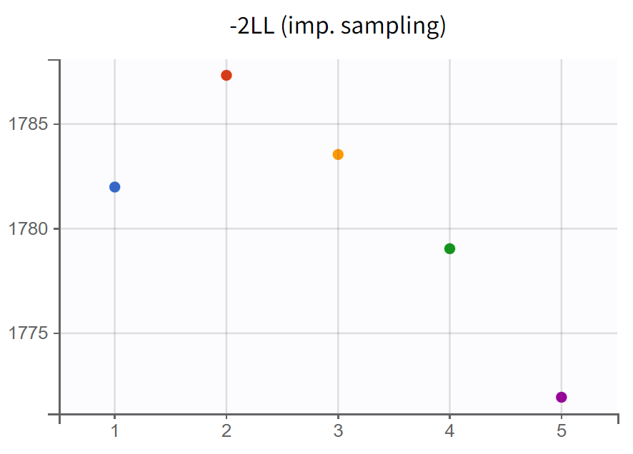
The turnover model (r02_4_1_turnover.mlxtran) shows varying likelihood values (). The trajectories indicate that fluctuates significantly upwards, which may be related to simulated annealing.

Note: Simulated annealing is enabled by default in Monolix to facilitate a broader exploration of the parameter space during the SAEM algorithm's exploration phase. By gradually decreasing the variance of random effects and residual error, it helps to increase the chances of finding a global optimum. However, this approach can also lead to upward fluctuations in the standard deviations of the random effects ().

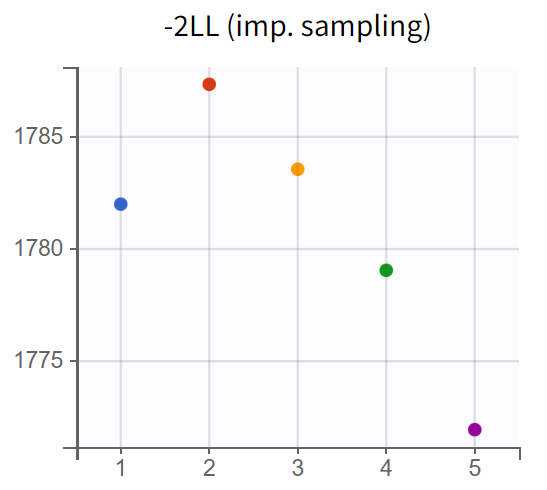
In the next step, the simulated annealing option in the population parameter estimation task is disabled, the auto-stop criterion is turned off, and the number of iterations in the exploration phase is increased from 500 to 1000. Extending the exploration phase allows more time to refine parameter estimates and prevents premature stopping, which can occur if convergence is detected too early, especially in complex models or noisy data. This ensures a more thorough exploration of the parameter space, leading to potentially more stable estimates.

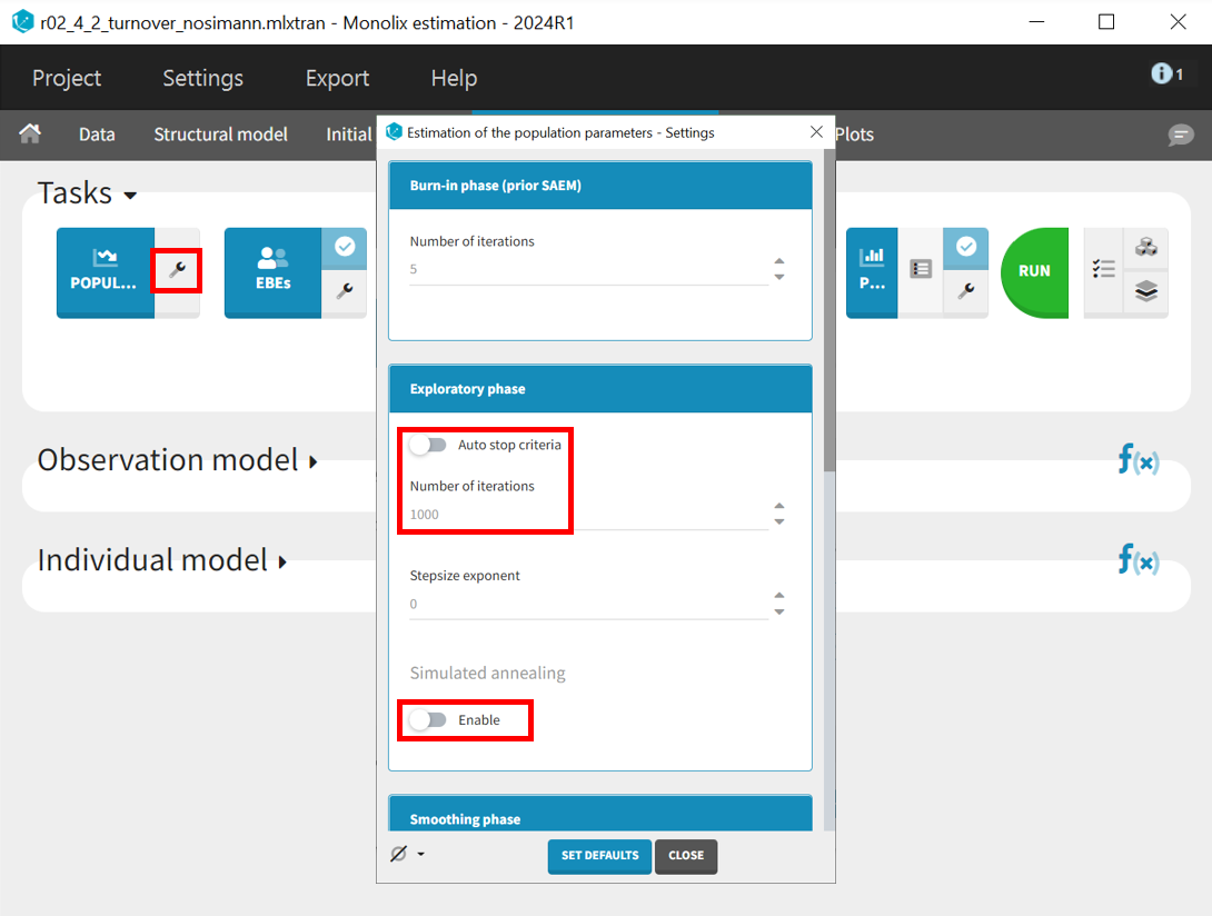
The project is saved under a new name (r02_4_2_turnover_nosimann.mlxtran) without carrying over the estimated values, ensuring that the initial values remain the same as in the previous run (r02_4_1_turnover.mlxtran). The estimation tasks and convergence assessment are then performed to evaluate the impact of the modified settings.

Turnover model without simulated annealing (r02_4_2_turnover_nosimann.mlxtran)	Tunover model with simulated annealing (r02_4_1_turnover.mlxtran)

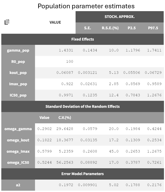
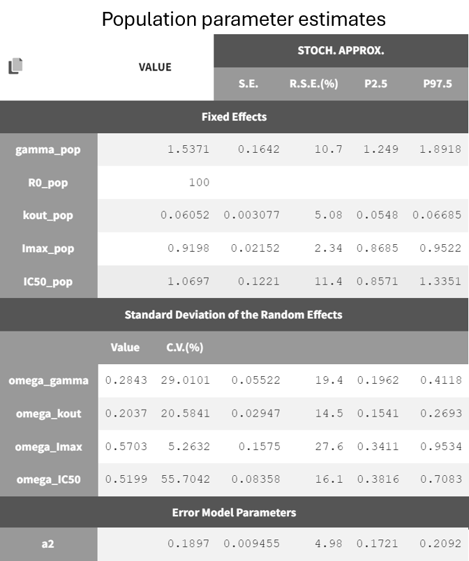
A comparison of the two models shows that the PD population parameter estimates are very similar, with relatively good certainty. The omega parameters do not become very small, and their RSEs increase, indicating that the random effects remain identifiable after disabling simulated annealing and that parameter variability should be retained. Disabling simulated annealing also reduces high oscillations in the trajectories of , leading to a smoother and more extended convergence, which results in a more stable likelihood. The model without simulated annealing leads to 4. No further improvements in stability are observed, making this the final PKPD model.

Simulations

The final Monolix model serves as a basis for simulations. The transition from estimations to simulations is seamless, facilitated by exporting the Monolix project to Simulx, where all estimates and the model are directly transferred.

Using this model, different treatment regimens can be simulated. The objective is to assess whether the proportion of subjects with PCA below 35% of baseline at 96 hours is significantly higher in the test arm, which receives 20 mg once daily for two days followed by 10 mg once daily, compared to the reference arm receiving 10 mg once daily. Each arm includes 100 individuals in a parallel trial design.

The new treatment regimens are specified in the “Definition” tab under the “Treatment” subtag. The group receiving the loading dose is labeled Group_withLoading, while the group receiving a consistent daily drug amount is labeled Group_noLoading. The following treatment elements are defined.

Group_withLoading	Group_noLoading

For the simulation, a new output vector is defined, extending well beyond 96 hours after the first administration. It is based on the prediction curve (prediction of PCA), starting at time 0 and ending at 336 hours. The time discretization grid is set to hours. This allows visualization of the output distribution curve over time, capturing multiple administrations and providing the PCA value at 96 hours.

The simulation scenario is defined as follows. The parameter element is set to the vector , which contains all population parameter estimates. The newly defined output vector , extending to 336 hours, is selected. Treatment definitions differentiate the groups: the group receiving the loading dose (Group_withLoading) includes the elements , representing 20 mg administrations at 0 and 24 hours, and , covering 10 mg administrations from 48 to 312 hours. The second group (Group_noLoading) receives only 10 mg administrations from 0 to 312 hours. Each group consists of 100 individuals. Since the simulated population exceeds the original study population size, the element is used to generate individual weight and age values while maintaining the same overall distribution.

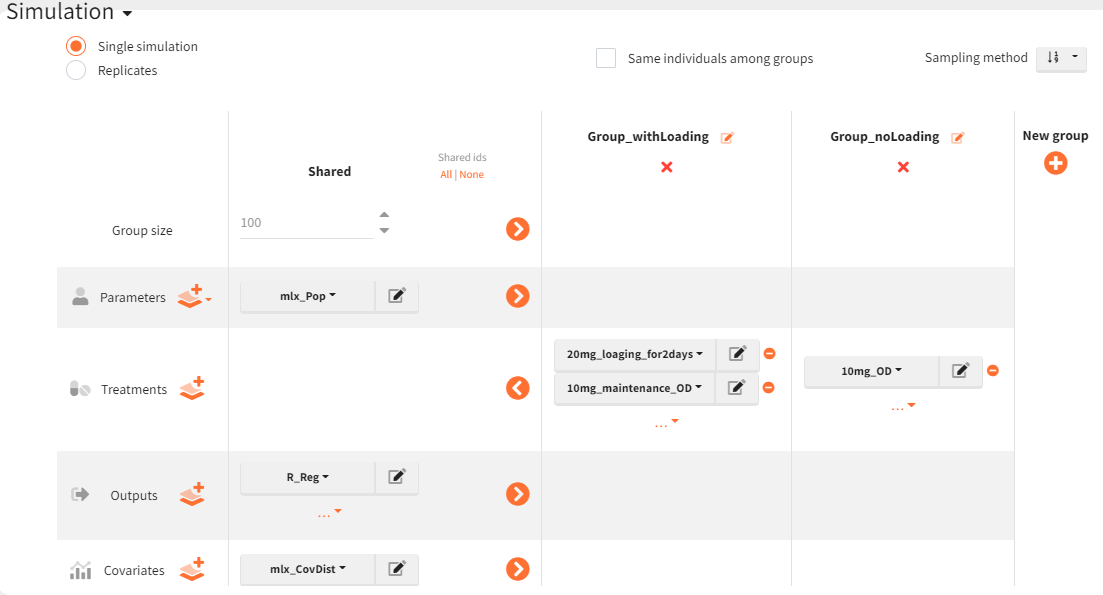
The Simulx project is saved under a new name (s01_simulation.smlx), and the simulation is conducted.

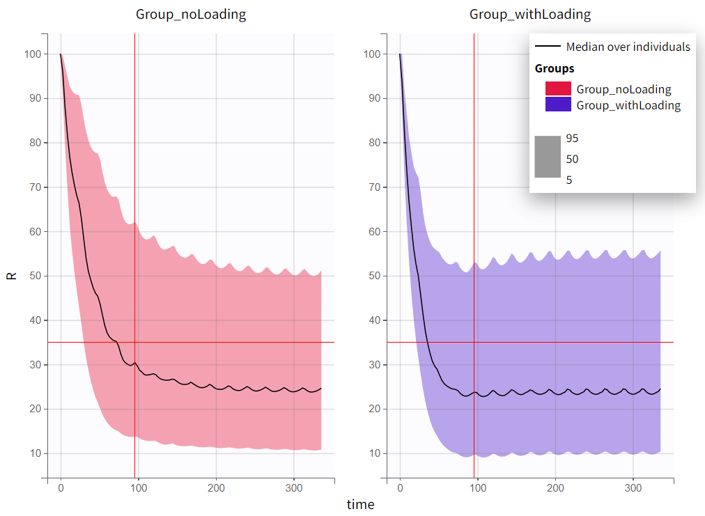
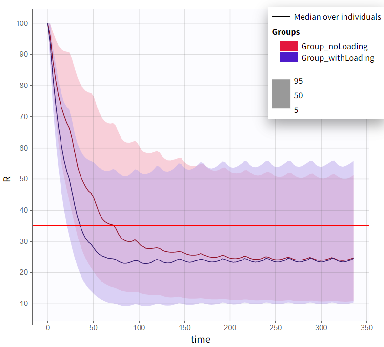
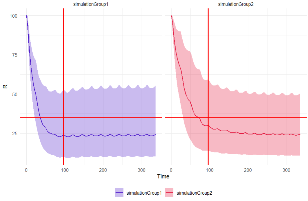
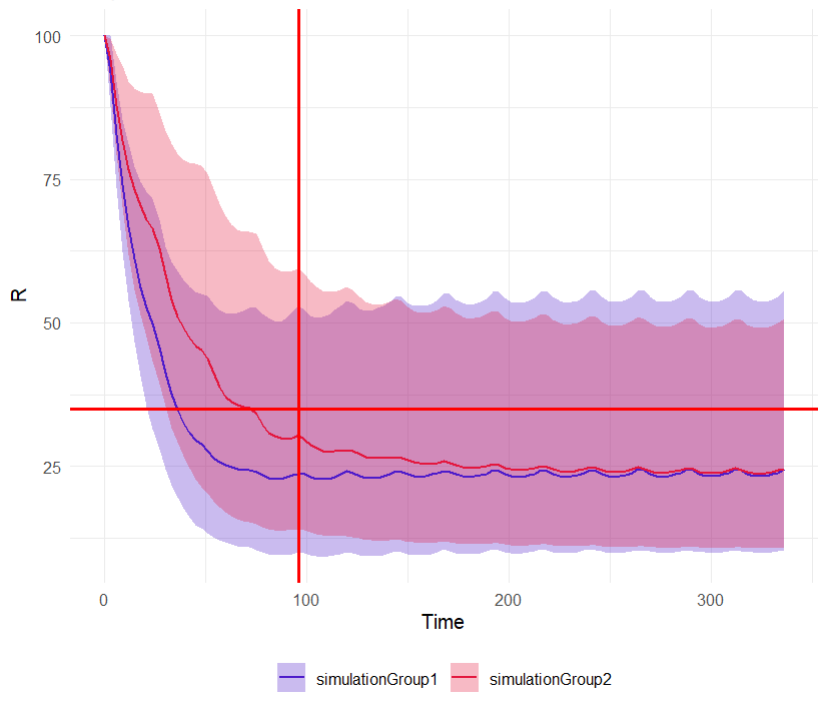
The output distribution plot displays the 5th, 50th, and 95th percentiles of the simulated data for all IDs. Visual cues at the time point of 96 hours (x=96h) and response level of 35% (y=35) show that both simulation groups have a median response below 35% at 96 hours. However, a substantial part of the percentile bands remains above this efficacy limit. The group receiving the loading dose reaches and stays below this threshold faster than the group without a loading dose.

The qualitative assessment suggests that the group with the loading doses performs better than the group without it. However, a quantitative comparison is required to confirm this observation. To achieve this, the simulation is post-processed by defining an outcome variable and summarizing it as an endpoint. The simulation groups can then be compared based on this endpoint.

The outcome is defined in the “Outcome & Endpoint” panel of the “Simulations” tab, representing a single value per subject. It is based on the prediction output vector . Custom value per ID is selected for output processing to extract the prediction at 96 hours. Additionally, a threshold is set to identify subjects with a predicted response below 35%, generating a boolean outcome: True for PCA values below 35% and False otherwise.

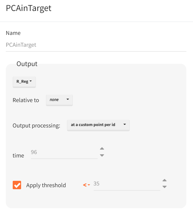
Once the outcome is created, an endpoint is automatically generated, summarizing the percentage of subjects in each simulation group for whom the result is True. Enabling the group comparison toggle allows for a statistical evaluation of differences between groups.

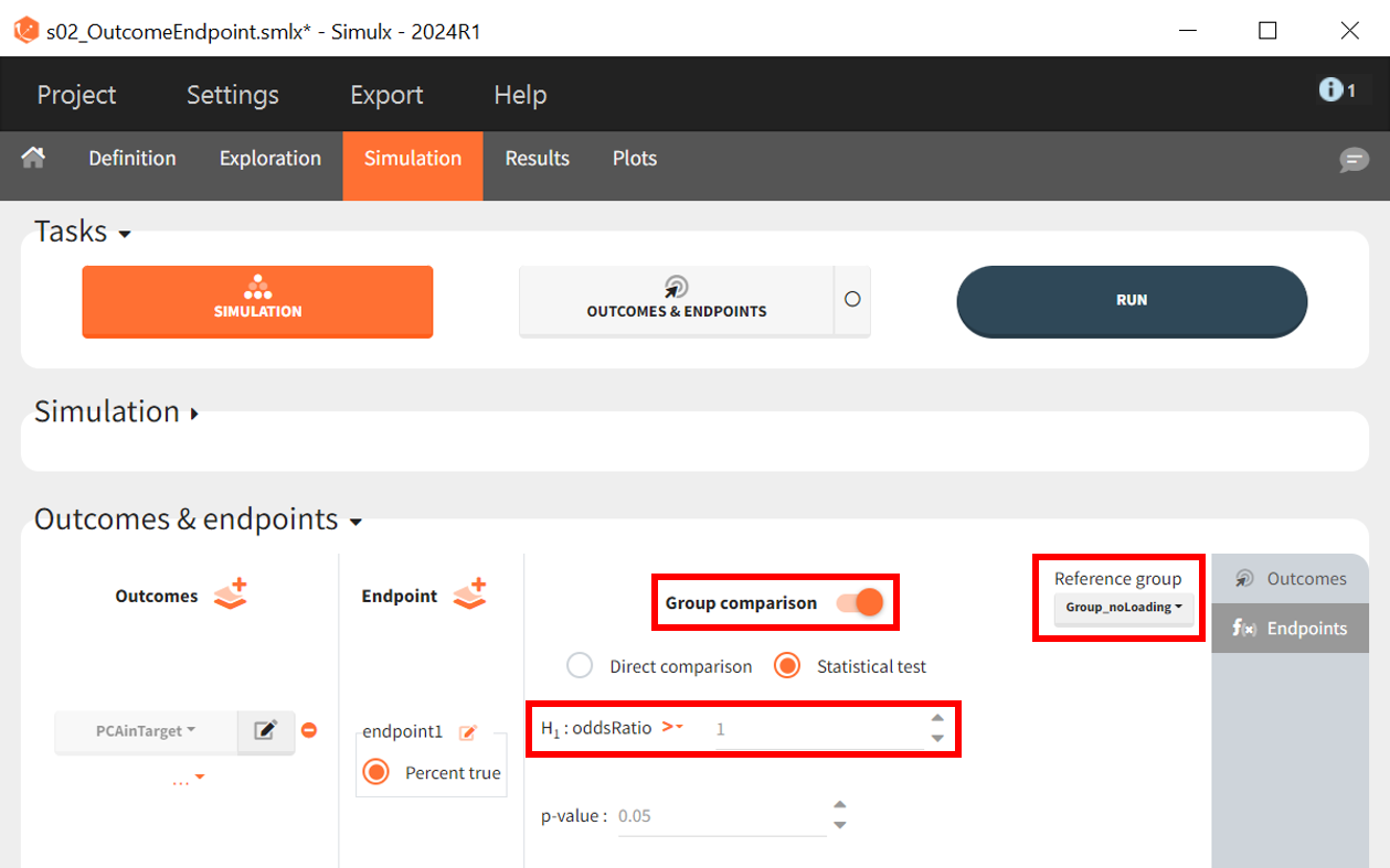
The statistical test applied is an odds ratio test using Fisher’s exact test. The objective is to determine whether the proportion of patients with PCA < 35% of baseline at 96 hours is significantly higher in the arm with the loading dose. The Group_noLoading arm is set as the reference group. The null hypothesis states that the reference group performs equally or better, implying a ratio 1, while the alternative hypothesis tests whether the Group_withLoading performs better, leading to an odds ratio > 1.

where and is the percentage of subject of their corresponding simulation group for which the condition holds true.

If the p-value is below 0.05, the null hypothesis is rejected in favor of the alternative hypothesis , indicating a successful trial.

The project is saved under a new name (s02_OutcomeEndpoint.slmx), and the outcome and endpoint task can be performed without rerunning the simulations, as the scenario remains unchanged.

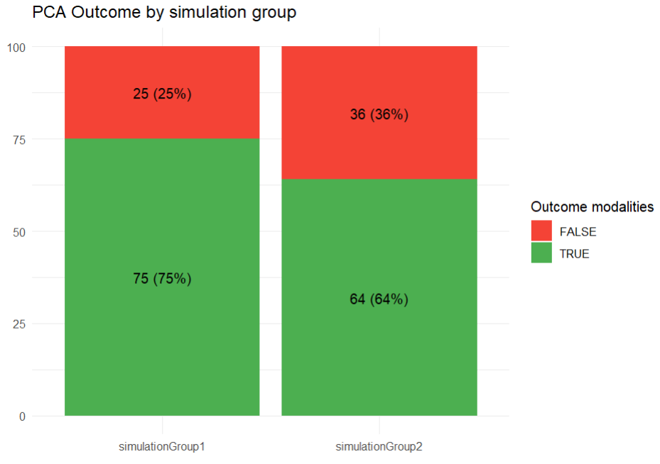
In the plots section, an outcome distribution plot is generated, displaying bar charts for each treatment group. These charts visually represent the number of subjects meeting the efficacy criteria versus those who do not.

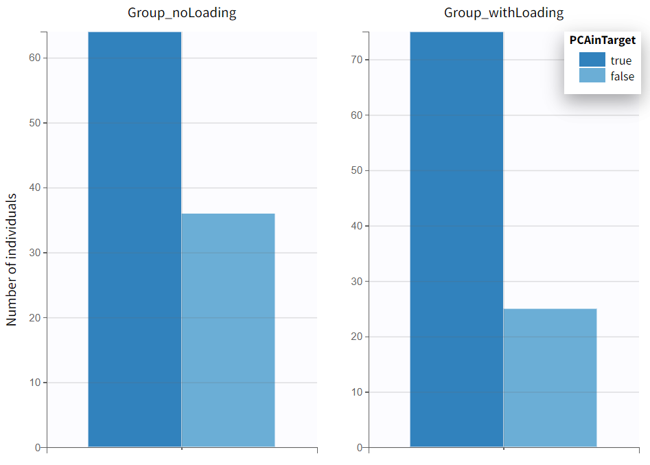
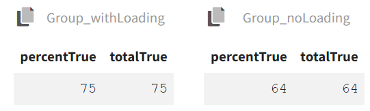
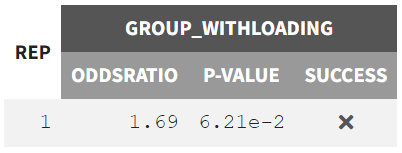
The results tab under the endpoint subtab shows the percentage of true outcomes per treatment group, with 75% in the Group_withLoading and 64% in the Group_noLoading. The group comparison subtab presents the results of the statistical odds ratio test. The difference between Group_withLoading and Group_noLoading is not statistically significant, though the p-value is borderline.

Odds per group	Group comparison

The smooth predictions based on ​ already indicate no clear significant difference between the treatment groups, suggesting that the expected population-level effect is minimal or absent. Given this outcome, further simulations incorporating noise through the response output vector​ and accounting for parameter uncertainty may not drastically alter the overall conclusion.

However, introducing variability could still provide insight into how much random fluctuations influence the results, particularly in equally sized or smaller sample sizes. If the goal is to evaluate whether the observed trend holds under realistic conditions, replicated simulations could be valuable. On the other hand, if the smooth model already offers a reliable estimate and the expected effect size is small, the additional complexity may not yield further insights.

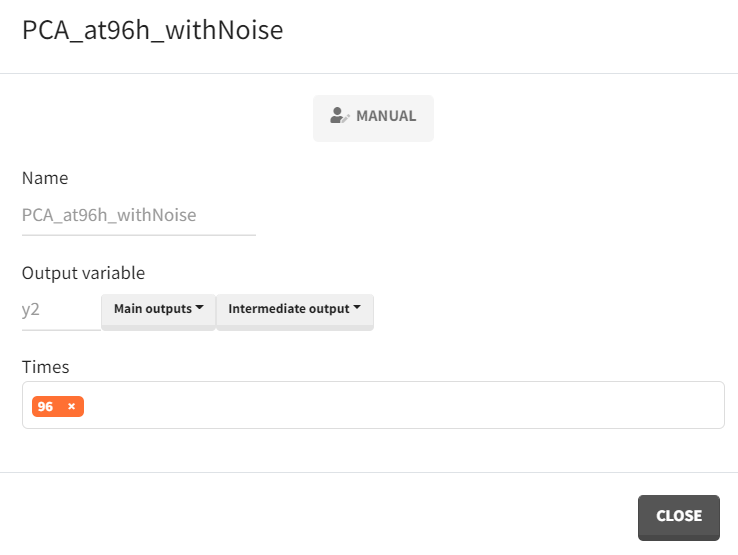
The simulation scenario requires some modifications. First, a new output vector must be created based on the observed PCA measurements. In the “Definition” tab under the output subtab, the observation vector , which consists of model predictions with an error model, replaces the smooth prediction vector as the basis. This time, only the 96-hour time point is of interest.

Next, the simulation scenario is set to replicates, with 20 experiment repetitions. The parameter element mlx_PopUncertain is selected, ensuring that the 20 simulations use different sets of population parameters to account for parameter uncertainty. Individual parameters in each replicate are drawn from these varying population parameters. The newly defined vector is selected as the output element.

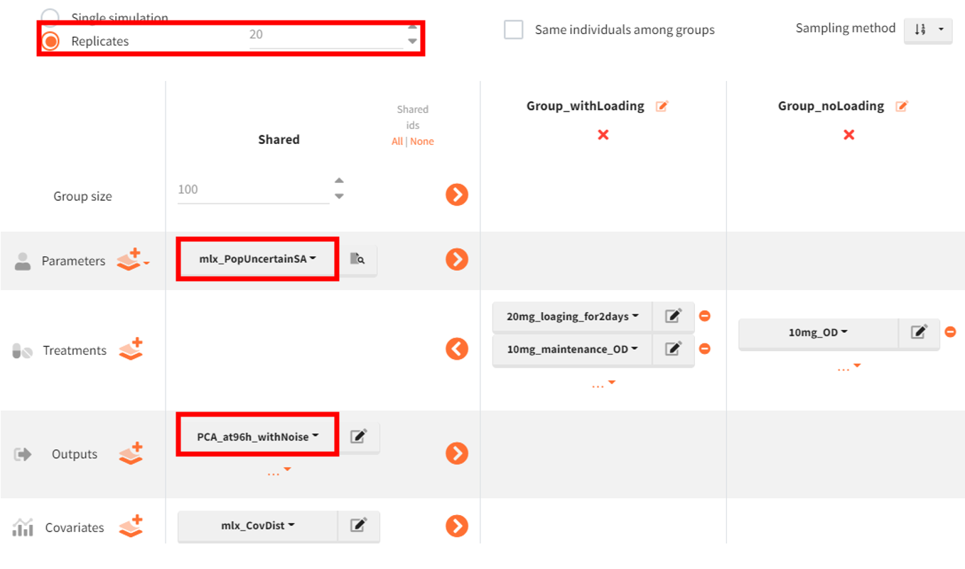
Finally, in the outcome & endpoint panel, the vector used for outcome calculations must be updated accordingly. The project is then saved under a new name (s03_ClinicalTrialReps.smlx), and simulations along with outcome and endpoint calculations are performed.

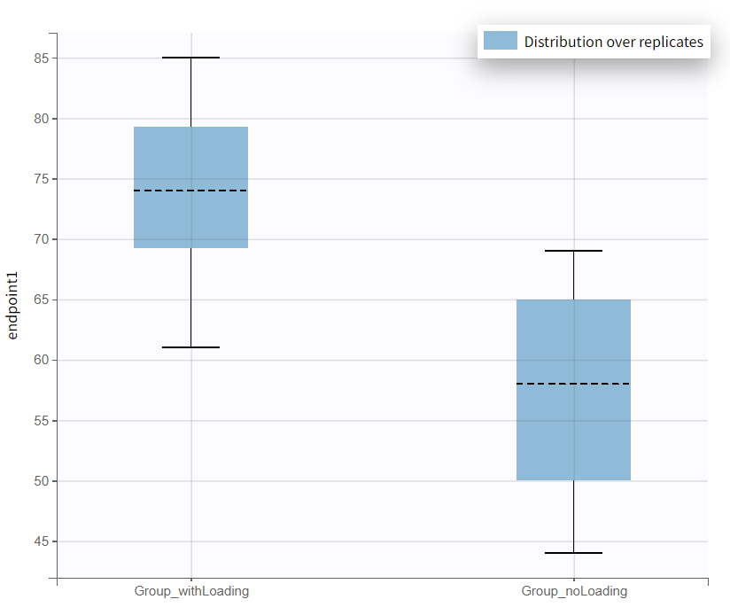
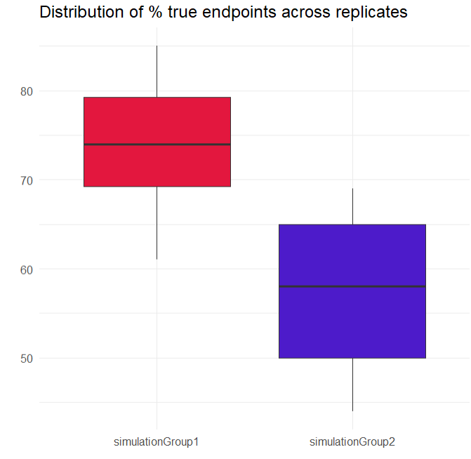
A new plot has been generated, summarizing the subjects who met the efficacy criterion across all replicates. Overall, Group_withLoading shows a higher median than Group_noLoading.

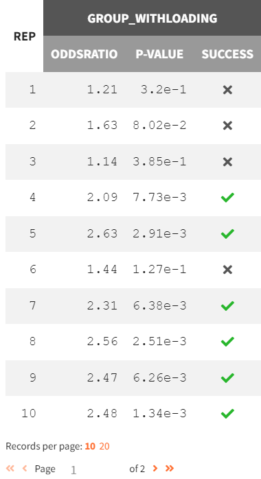
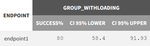
In the “Results” tab, the “Group Comparison” subtab presents a table with the statistical evaluation of the 20 comparisons. The "Summary" section displays the power of the clinical trial. Repeating the trial 20 times, incorporating noisy PCA measurements and population parameter uncertainty, results in a success rate of 80%.

Group comparison of 20 replicates	Success rate over all 20 replicates

Simulations using lixoftConnectors

All steps for setting up and executing the simulation scenario can be scripted one-to-one using the lixoftConnectors in R. The exact same approach is used as in the Simulx GUI.

First, a Monolix project is either exported or imported, followed by the definition of different treatment arms via the connector defineTreatmentElement():

• Group with loading dose: 20 mg at time 0 and 24 h (2 doses) & 10 mg from 48 h to 312 h with an interdose interval of 24 h (12 doses).

• Group without loading dose: 10 mg from time 0 to 312 h with an interdose interval of 24 h (14 doses).

Next, the output vector is defined by defineOutputElement() based on the smooth predictions of the response vector , extending to 336 h with an equidistant time discretization of 3 h.

rm(list = ls())
path.prog <- suppressWarnings(dirname(rstudioapi::getSourceEditorContext()$path))
setwd(path.prog)

# GOAL: Simulate treatment scenarios in Simulx to assess outcomes across different treatment groups

path.software <- paste0("C:/Program Files/Lixoft/MonolixSuite2024R1") 
install.packages(paste0(path.software,"/connectors/lixoftConnectors.tar.gz"), repos = NULL, type="source", INSTALL_opts ="--no-multiarch")
library(lixoftConnectors)

# software initialization: specify the software to be used
initializeLixoftConnectors(path.software,software = "monolix")

# loading the final Monolix project
path.project <- paste0(path.prog,"/r02_4_2_turnover_nosimann.mlxtran")
loadProject(projectFile = path.project)

# export monolix project to simulx
exportProject(settings = list(targetSoftware = "simulx", filesNextToProject = T), force=T)

# definition of the new treatment regimen
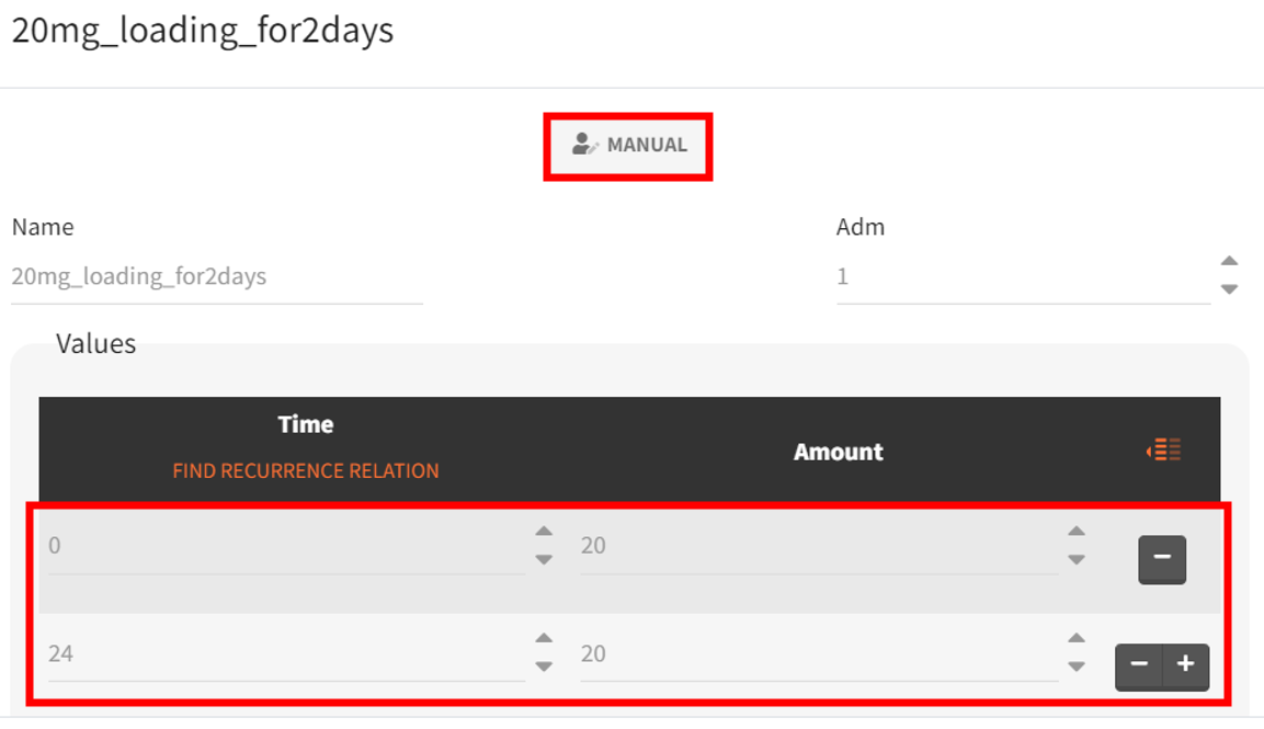
defineTreatmentElement(name = "20mg_loading_for2days", element = list(data=data.frame(start=0 , interval=24, nbDoses=2 , amount=20)))
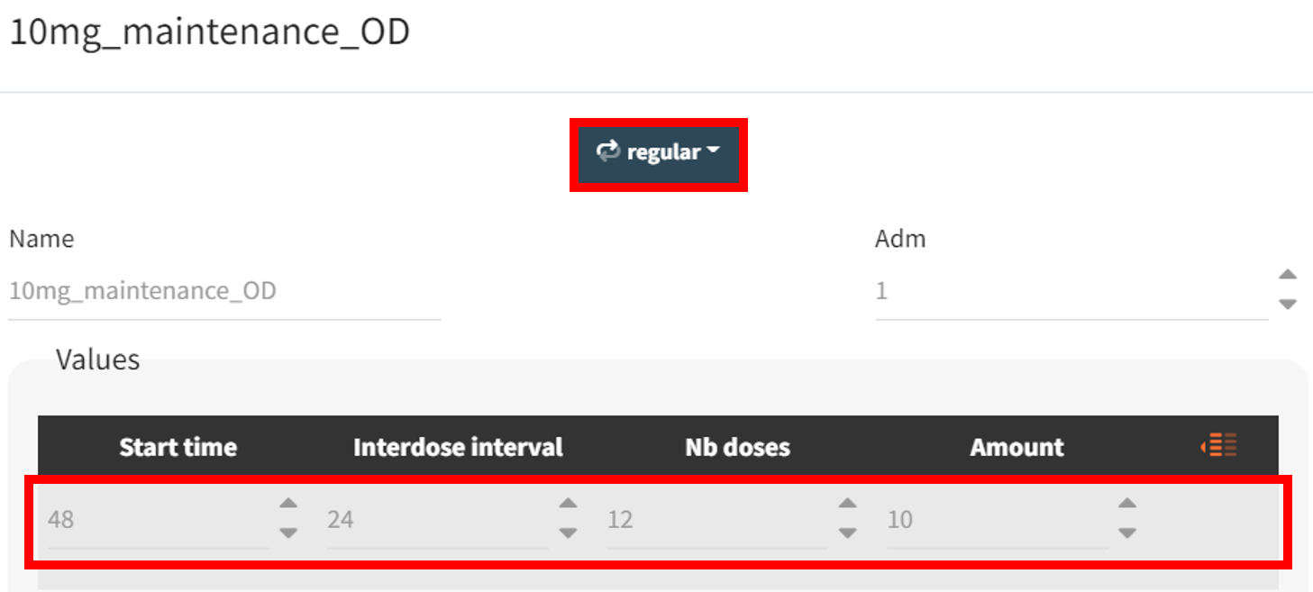
defineTreatmentElement(name = "10mg_maintenance_OD"  , element = list(data=data.frame(start=48, interval=24, nbDoses=12, amount=10)))
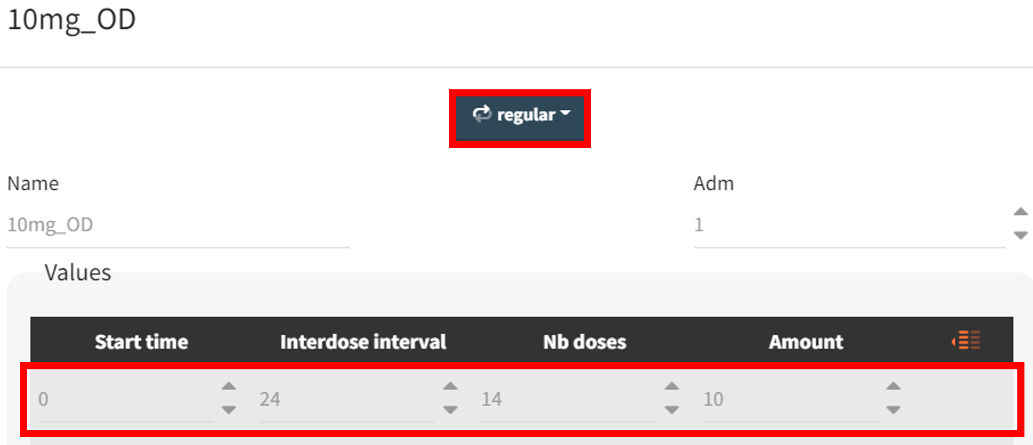
defineTreatmentElement(name = "10mg_OD"              , element = list(data=data.frame(start=0 , interval=24, nbDoses=14, amount=10)))

# definition of the output vector
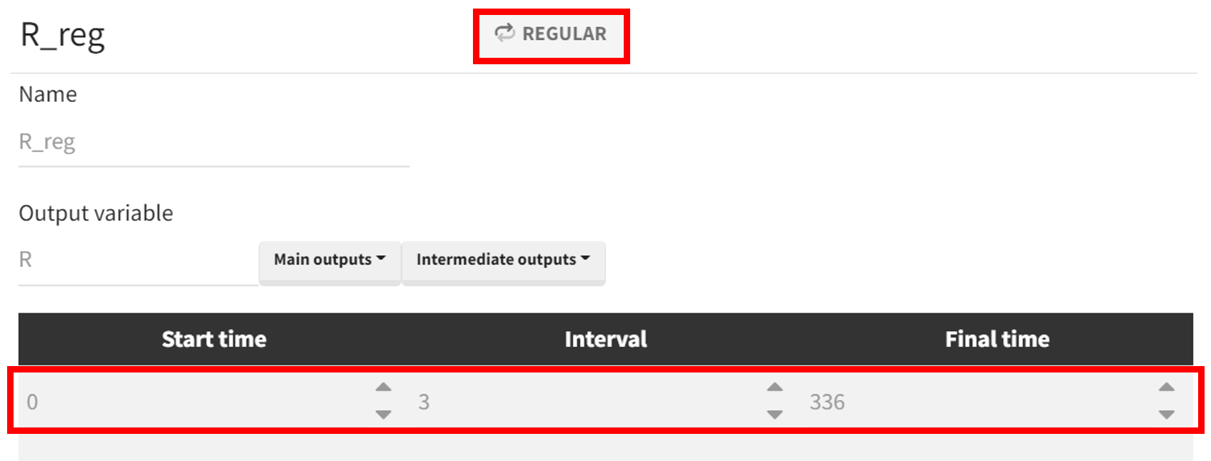
defineOutputElement(name = "R_Reg", element = list(data = data.frame(start = 0, interval = 3, final = 336), output = "R"))

The simulation scenario is then specified with setGroupElement(), incorporating the two treatment groups with different dosing regimens while maintaining the same group size, parameter element mlx_Pop, output vector R_Reg, and covariate element mlx_CovDist.

The outcome and endpoint are defined via the connectors defineOutcome() & defineEndpoint() before running the simulation. The outcome for each subject is determined based on whether the criterion PCA(96h) < 35% is met. If satisfied, the subject is assigned true; otherwise, false. The results are then summarized using the endpoint and statistically compared. An odds ratio test (Fisher’s exact test) is applied, using Simulation Group 2 as the reference. The goal is to assess whether simulationGroup1 meets the efficacy criterion significantly more often.

# simulation scenario setup
setGroupElement(group = "simulationGroup1", elements = c("mlx_Pop"))
setGroupElement(group = "simulationGroup1", elements = c("R_Reg"))
setGroupElement(group = "simulationGroup1", elements = c("mlx_CovDist"))
setGroupElement(group = "simulationGroup1", elements = c("20mg_loading_for2days","10mg_maintenance_OD"))
setGroupSize("simulationGroup1",100)
addGroup("simulationGroup2")
setGroupElement(group = "simulationGroup2", elements = c("10mg_OD"))

# outcome definition
defineOutcome(name = "PCAinTarget", element = list(output = "R_Reg", processing = list(operator = "timePoint", value =96),applyThreshold = list(operator = "<", threshold = 35))) 

# endpoint definition 
defineEndpoint(name    = "TreatmentComparison_OR_test", 
               element = list(outcome         = "PCAinTarget",  
                              metric          = "percentTrue",
                              groupComparison = list(type      = "statisticalTest", 
                                                     operator  = ">", 
                                                     threshold = "1", 
                                                     pvalue    = 0.05)))
# set reference group
setGroupComparisonSettings(referenceGroup = "simulationGroup2", enable = TRUE)

# configure simulation and endpoint calculation
setScenario(c(simulation = T, endpoints = T))
runScenario()

The simulation results can be retrieved via getSimulationResults() and written as a data frame. A few lines of code create the output distribution plot, but calculating the percentiles of the simulated response curves requires loading the dplyr package. Diagnostic plots can be constructed using ggplot. The last line is optional and splits the simulation group plots; commenting it out merges the split plots.

# retrieve simulation results
sim_results <- data.frame(getSimulationResults()$res$R)

library(dplyr)
# Compute percentiles
summary_data <- sim_results %>%
  group_by(time, group) %>%
  summarise(p5  = quantile(R, 0.05), # 5th percentile
            p50 = quantile(R, 0.50), # Median
            p95 = quantile(R, 0.95), # 95th percentile
            .groups = "drop")

library(ggplot2)
# create output distribution plot distinct by simulation groups
output_distrib <- ggplot(summary_data, aes(x = time, group = group, fill = group)) +
  geom_ribbon(aes(ymin = p5, ymax = p95, fill = group), alpha = 0.3) +
  geom_line(aes(y = p50, color = group), linewidth = 0.7) +
  geom_vline(xintercept = 96, color = "#FF0000", linetype = "solid", linewidth = 0.8) + # vertical line at 96h
  geom_hline(yintercept = 35, color = "#FF0000", linetype = "solid", linewidth = 0.8) + # horizontal line at 35% response
  scale_color_manual(values = c("simulationGroup1" = "#4D1BCA", "simulationGroup2" = "#E3173E")) +
  scale_fill_manual(values = c("simulationGroup1" = "#4D1BCA", "simulationGroup2" = "#E3173E")) +
  labs(x = "Time", y = "R", title = "Output distribution") +
  theme_minimal() +
  theme(legend.title = element_blank(), legend.position = "bottom") 
  # facet_wrap(~group)

The outcome and endpoint results can also be retrieved as a data frame by getEndpointsResults(). The following code summarizes the outcome results using a stack chart, which visualizes the endpoint results.

# retrieve outcome and endpoint results
res_PCAinTarget    <- data.frame(getEndpointsResults()$outcomes$PCAinTarget)
res_Endpoint       <- data.frame(getEndpointsResults()$endpoints$TreatmentComparison_OR_test)
res_TrtmComparison <- data.frame(getEndpointsResults()$groupComparison$TreatmentComparison_OR_test)

# Calculate the count of TRUE and FALSE for each simulation group
summary_data <- res_PCAinTarget %>%
  group_by(group) %>%
  summarise(TRUE_count  = sum(PCAinTarget == TRUE),
            FALSE_count = sum(PCAinTarget == FALSE),
            total       = n()) %>%
  tidyr::pivot_longer(cols      = c(TRUE_count, FALSE_count), 
                      names_to  = "outcome", 
                      values_to = "count") %>%
  mutate(outcome    = ifelse(outcome == "TRUE_count", "TRUE", "FALSE"),
         percentage = count / total * 100)

# Create the stacked bar chart
outcome_distrib <- ggplot(summary_data, aes(x = group, y = count, fill = outcome)) +
  geom_bar(stat = "identity", position = "stack") +
  geom_text(aes(label = paste0(count, " (", round(percentage, 1), "%)")), 
            position = position_stack(vjust = 0.5)) +
  labs(title = "PCA Outcome by simulation group", x = "", y = "", fill = "Outcome modalities") +
  theme_minimal() +
  scale_fill_manual(values = c("TRUE" = "#4CAF50", "FALSE" = "#F44336"))

The final step involved simulating a clinical trial and repeating the experiment 20 times. This introduced more noise into the response and accounted for population parameter uncertainty. The definition of treatment arms remains unchanged, but the output vector and therefore also the outcome need to be redefined.

# definition of the output vector
defineOutputElement(name = "PCA_at96h_withNoise", element = list(data = data.frame(time=96), output = "y2"))

The simulation scenario must incorporate the parameter element mlx_PopUncertainSA and the new output vector PCA_at96h_withNoise, while all other settings remain the same.

# simulation scenario setup
setGroupElement(group = "simulationGroup1", elements = c("mlx_PopUncertainSA"))
setGroupElement(group = "simulationGroup1", elements = c("PCA_at96h_withNoise" ))
setGroupElement(group = "simulationGroup1", elements = c("mlx_CovDist"))
setGroupElement(group = "simulationGroup1", elements = c("20mg_loading_for2days","10mg_maintenance_OD"))
setGroupSize("simulationGroup1",100)
addGroup("simulationGroup2")
setGroupElement(group = "simulationGroup2", elements = c("10mg_OD"))

# outcome definition
defineOutcome(name = "PCAinTarget", element = list(output = "PCA_at96h_withNoise", processing = list(operator = "none"), applyThreshold = list(operator = "<", threshold = 35))) 

The number of repetitions must be explicitly specified with setNbReplicates().

Once these adjustments are made, the simulations can be executed.

# retrieve outcome and endpoint results
res_Endpoint <- data.frame(getEndpointsResults()$endpoints$TreatmentComparison_OR_test)

# Create boxplots
boxplots <- ggplot(res_Endpoint, aes(x = group, y = percentTrue, fill = group)) +
  geom_boxplot()+
  scale_fill_manual(values = c("simulationGroup1" = "#E3173E", "simulationGroup2" = "#4D1BCA")) +
  labs(title = "Distribution of % true endpoints across replicates", x = "", y = "") +
  theme_minimal() +
  theme(legend.position = "none")

Discussions and conclusions

The model development process required several steps to ensure not only a good model fit but also stable and robust estimates. The convergence assessment proved valuable in verifying whether seemingly reliable estimates were truly reproducible.

Simulations indicated that the treatment group with a loading dose showed no statistically significant effect compared to the schedule without a loading dose. The applied test compared the odds of meeting the efficacy criterion PCA(96h) < 35%, with a borderline p-value suggesting a possible trend.

Although the initial experiment, based on smooth prediction response curves and stable estimates, showed no significant treatment group difference, simulating a clinical trial with added noise and uncertainty and repeating it multiple times provided further insights. The conclusion is that in 80% of repetitions, the loading dose treatment arm was statistically significantly superior to the treatment arm without a loading dose based on the efficacy criterion.