Download data set only | Download Monolix project files
In this example NCA, CA and popPK workflow, we introduce inter-occasion variability to analyse the absorption and elimination of alcohol with or without a dietary additive of guar gum.
Guar gum, also called guaran, is a polysaccharide extracted from guar beans. As a natural polymer, it has been used for many years as an emulsifier, thickener, and stabilizer in the food industry. In the pharmaceutical sector, guar gum and guar-gum based systems are frequently studied for the development of controlled-released formulations and colon targeted drug delivery systems, as guar gum can protect active molecules from the enzymes and pH in the stomach and small intestine and it can be degraded by intestinal bacteria in the colon. [Aminabhavi, T. M., Nadagouda, M. N., Joshi, S. D., & More, U. A. (2014). Guar gum as platform for the oral controlled release of therapeutics. Expert Opinion on Drug Delivery, 11(5), 753–766.]
Moreover, guar gum may affect the bioavailability of concomitantly administered substances due to its effect on the rate of gastrointestinal transit and gastric emptying.
The goal of this case study is then to assess the effect of guar gum on the absorption and bioavailability of alcohol.
Outline:
Data set
The data has been published in:
Practical Longitudinal Data Analysis, David J. Hand, Martin J. Crowder, Chapman and Hall/CRC, Published March 1, 1996
It is composed of measurements of blood alcohol concentrations in 7 healthy individuals. All subjects took alcohol at time 0 and gave a blood sample at 14 times over a period of 5 hours. The whole procedure was repeated at a later date but with a dietary additive of guar gum. The two different periods of time are encoded in the data with overlapping times, both starting at time 0.
Although the precise amount of ingested alcohol is unknown, for this case study we assume each amount to be 10g (standard drink).
Data Exploration in PKanalix

The data is loaded into PKanalix for graphical exploration, as shown in the screenshot. In the Data tab, time is in hours, alcohol concentration in the Y column is in mg/L, and the amount in the AMT column is in mg. Censored observations are indicated with the column CENS tagged as CENSORING.
The two measurement periods, during which subjects either received guar gum with alcohol or not, are distinguished by the column OCC, which is automatically recognized as OCCASION. Additionally, the column DIET is tagged as CATCOV to specify which period included guar gum. This column contains two values: "noGuar" for the first period and "withGuar" for the second period.
In the Plots tab, the graph of alcohol concentration versus time on log-scale seen below indicates to use a one-compartment model with first-order absorption. While some individuals show non-linear elimination, the data may be insufficient to fully capture this. Therefore, a linear elimination model should be considered as an initial approach.
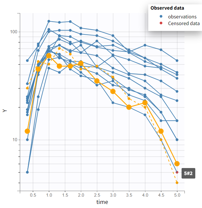
The different occasions can be visualized in several ways. First, hovering on a curve highlights the curve in solid yellow and the curve corresponding to the other occasion from the same subject in dashed yellow, as on the figure above.
Second, OCC is available for stratification along with the covariate DIET in the “Stratify” panel , and can thus be used for splitting, coloring or filterting. Below are for example the subplots of the data split by OCC and colored by ID. Each subject-occasion is assigned a color, with matched color shades for subject-occasions corresponding to the same subject. This is convenient to compare at a glance the two occasions for all subjects.
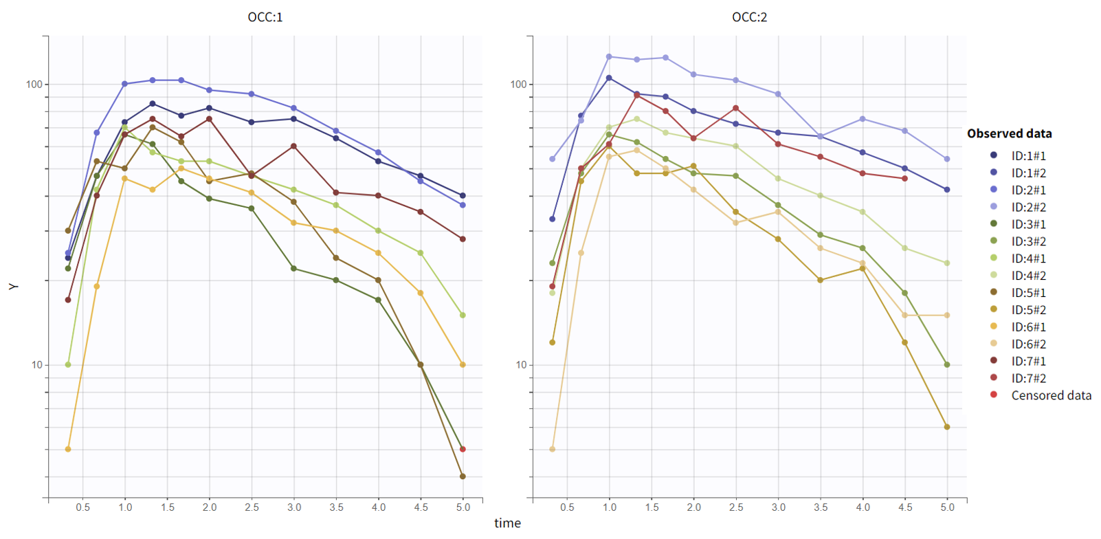
The inter-individual variability seems mostly reproduced from one occasion to the other, and concentration levels seem slightly higher for OCC=2.
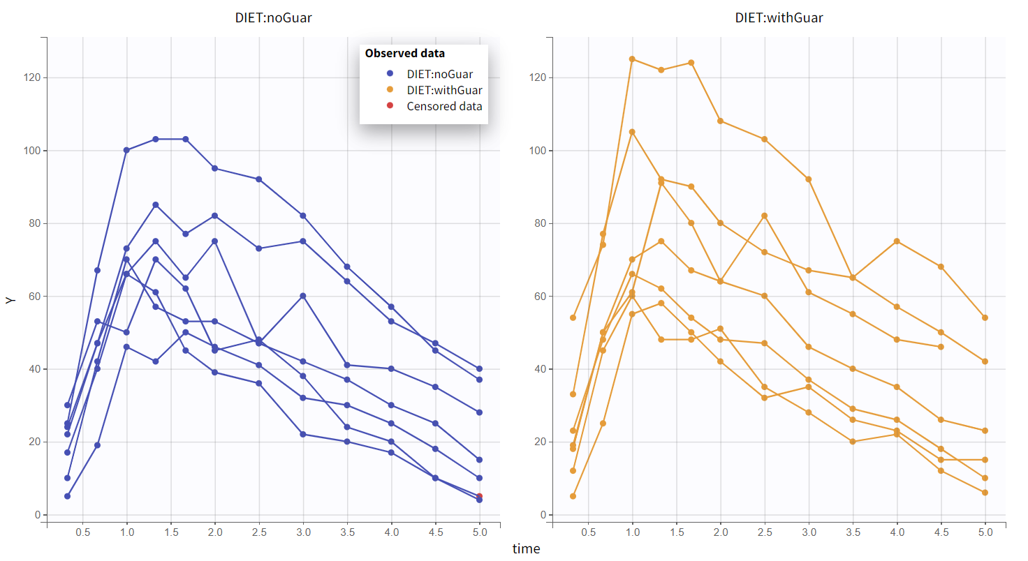
This global trend is further confirmed in the linear scale plot shown below. The plot is color-coded by DIET, with categories aligned to OCC: DIET="noGuar" corresponds to OCC=1, and DIET="withGuar" to OCC=2. As a result, the primary inter-occasion variability observed in the data appears to be driven by the covariate DIET.
Analysis in PKanalix
Non-compartmental analysis
As an initial analysis, we will examine the difference in PK parameters between the two occasions using non-compartmental analysis (NCA) in PKanalix. Since we are already in PKanalix, simply navigate to the Task tab under the NCA section, and apply the following settings:
-
extravasuclar as administration type,
-
“linear up log down” as AUC integartion method
-
“missing“ for blq after Tmax (censored observations after Tmax are not used in the analysis)
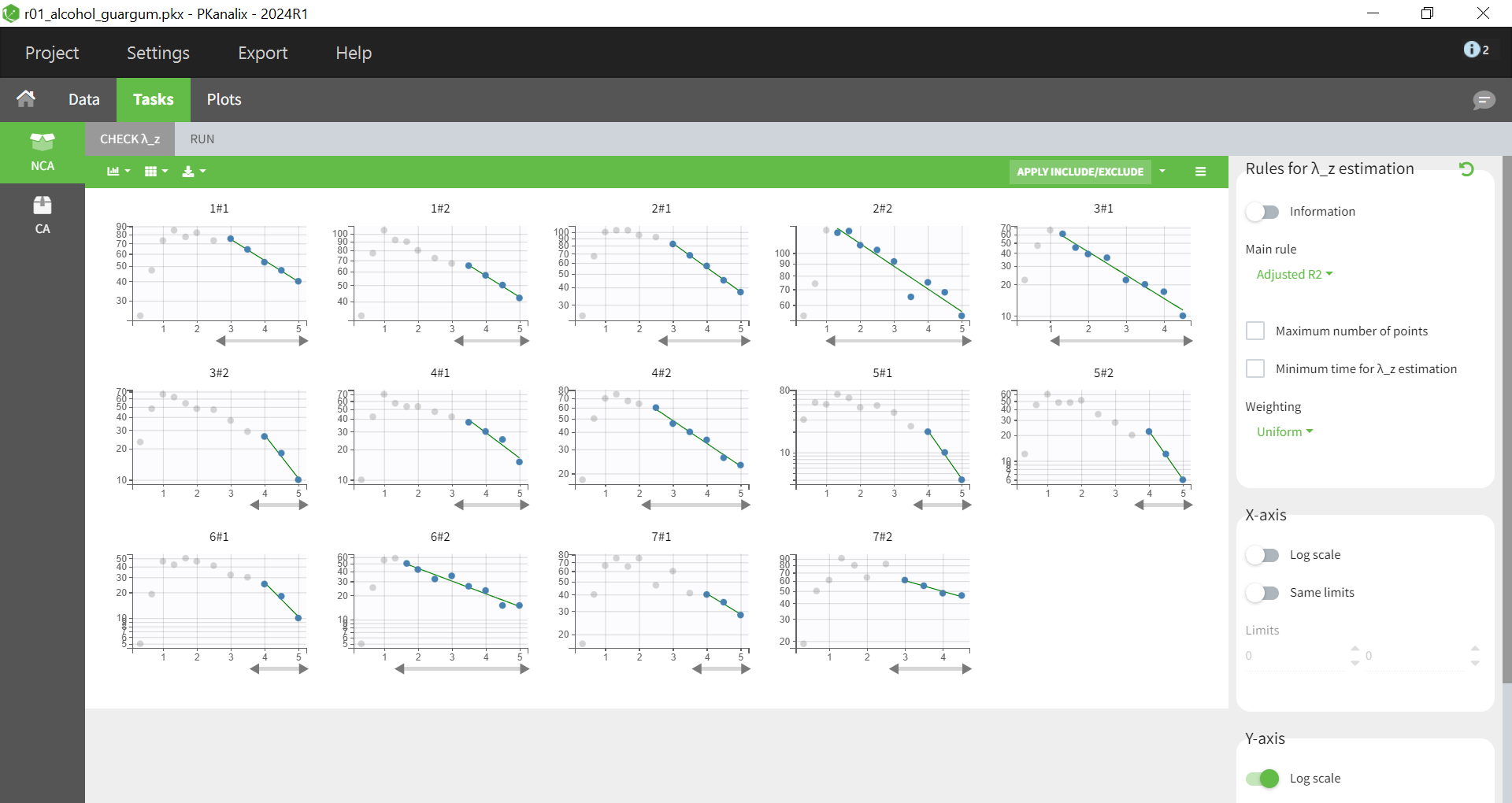
The "Check lambda_z" panel, shown below, enables the assessment of regressions used to estimate the terminal slope. By default, the "adjusted R²" criterion is applied to select the optimal number of data points for each individual, ensuring the best possible regression fit. While the plots provide an option to manually adjust the point selection for certain individuals, this adjustment is unnecessary in this case. The plots already reveal variability in the estimated lambda_z across individuals.
Running the NCA gives the lambda_z and other PK parameters for each individual. In the “Plot” tab, the plot of individual parameters vs. covariates is convenient to visualize the variability in the parameters and compare the distributions without and with guar gum. Here the following parameters have been selected: AUCINF_pred, Cl_F_pred, Cmax, HL_Lambda_z, Tmax:
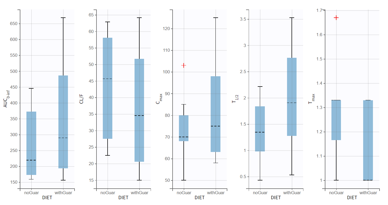
Differences between the two modalities are noticeable for half-life, clearance, and Cmax. However, there is lagre variability in these parameters within each dietary condition.
Compartmental analysis in PKanalix
Next, a compartmental analysis (CA) is performed to estimate a compartmental model and compare the parameters between the two conditions. PKanalix treats each subject-occasion as independent, optimizing the parameters separately for each individual and each occasion. This approach facilitates an easy comparison of parameter estimates across the two occasions.
Selecting a one-compartment model with first-order absorption and linear elimination yields the following individual fits (after setting initial values using the "aut-init" button):
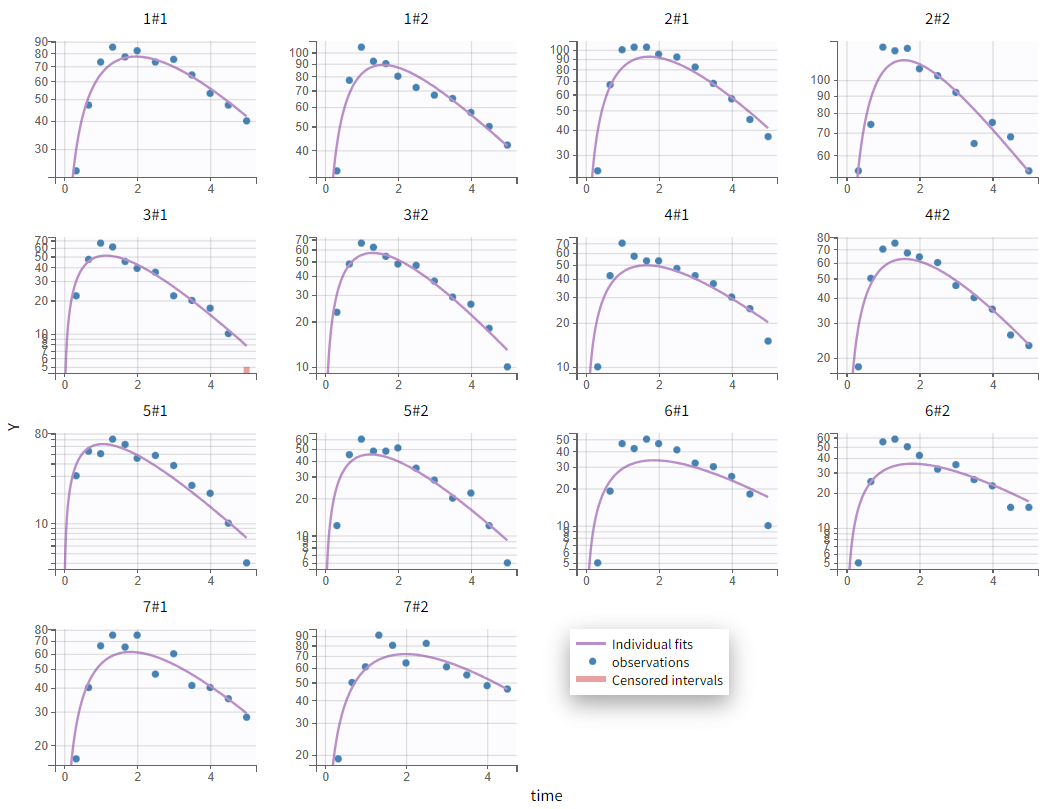
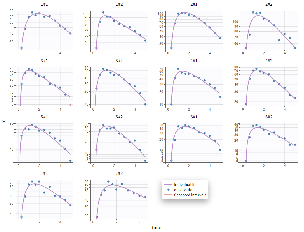
The absorption phase is not well captured in the current model. Zooming in on the early phase suggests that a delay in absorption should be considered, as the first observed data point is consistently overpredicted. Applying the same model with an added lag time before absorption provides more accurate individual fits:
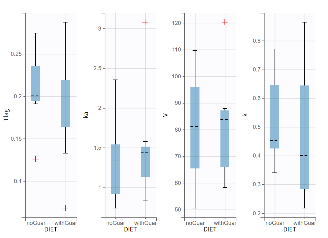
In the plot Individual parameters vs. covariates, the estimated individual parameters show different distributions across the two conditions of DIET, in particular for ka, V and k:
Given the small size of the dataset, it is uncertain whether the observed differences are statistically significant. A more precise assessment of the effect of DIET on alcohol kinetics can be achieved through a detailed population analysis in Monolix.
Additionally, the current model does not explicitly account for bioavailability, as it is not identifiable with only extravascular administrations and is thus included in the apparent volume, V. Monolix offers the capability to utilize more complex models beyond the basic PK models available in the library, including the explicit incorporation of bioavailability. This allows for a more meaningful evaluation of whether guar gum affects the relative bioavailability in relation to DIET.
Consequently, the compartmental model will be exported from PKanalix to Monolix for further analysis.
Population modelling in Monolix
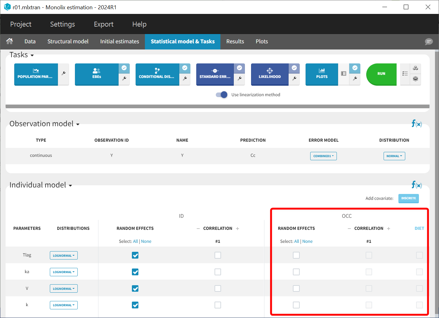
In the "Statistical Model & Tasks" tab, the "Individual Model" section is now divided into two components. The left side, at the ID level, addresses inter-individual variability (IIV) and includes a default random effect for each parameter. The right side (highlighted in the figure below) focuses on inter-occasion variability (IOV) and allows for the addition of random effects at the inter-occasion level. Since DIET varies across occasions, it is included in this panel to account for part of the IOV through a covariate effect. The covariate effect boxes are currently greyed out because no inter-occasion variability has been specified at this stage. Covariate effects can only be added at the occasion level to parameters that either exhibit IOV with random effects at the occasion level or have no random effects at the ID and occasion levels.
Model without inter-occasion variability
The first step in this workflow focuses on validating the structural model without accounting for differences between occasions. The statistical model is kept at its default settings, all tasks in the scenario are selected, and the project is saved as run01.mlxtran.
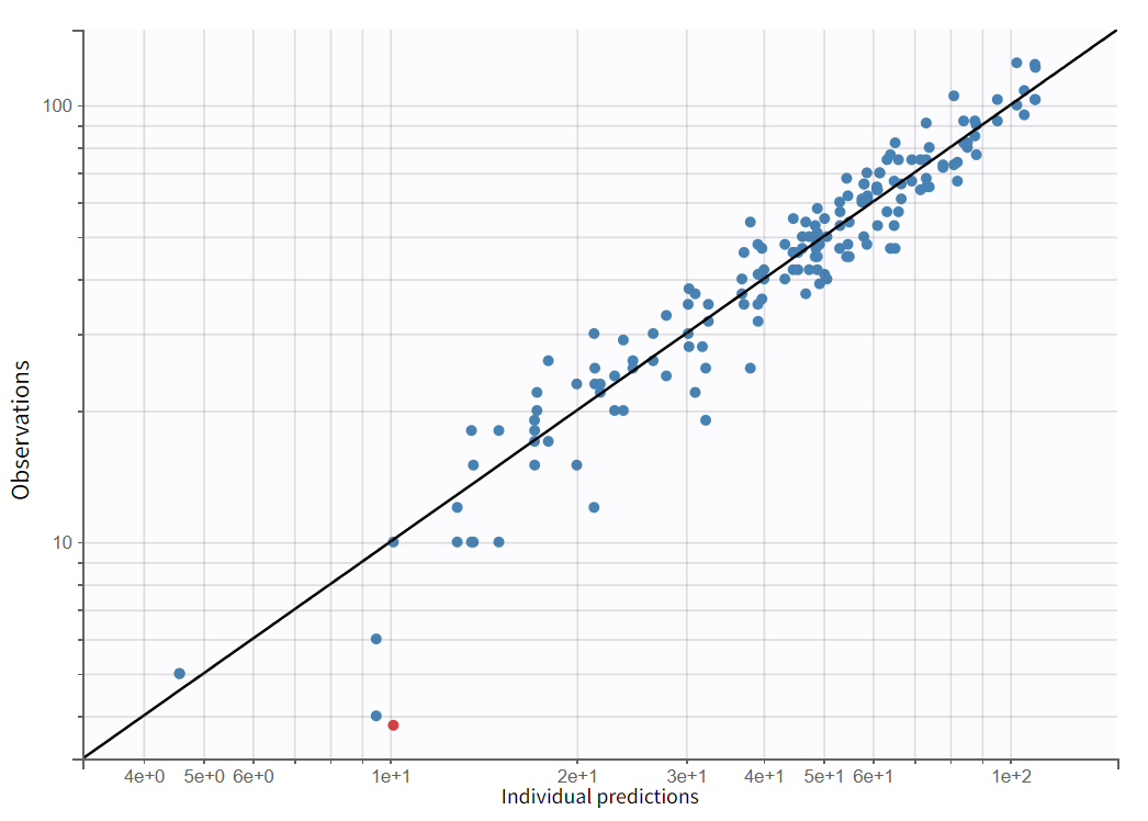
Estimating this model reveals no misspecifications, as evidenced by the plot of Observations versus Predictions in a log-log scale. Upon estimating the model, no obvious misspecifications are apparent. However, some data points are clustered significantly below the identity line, reflecting an overprediction. Hovering over these points shows that most of them correspond to early time points.
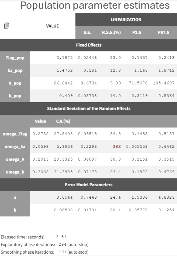
All parameters were estimated with good confidence, except for omega_ka which is very small with a very high relative standard error:
On the individual fits seen below, disabling the option “Split occasions” in “Display” allows to visualize the two occasions on the same plot for each individual. The observed data can be colored by occasion or equivalently by DIET in Stratify.
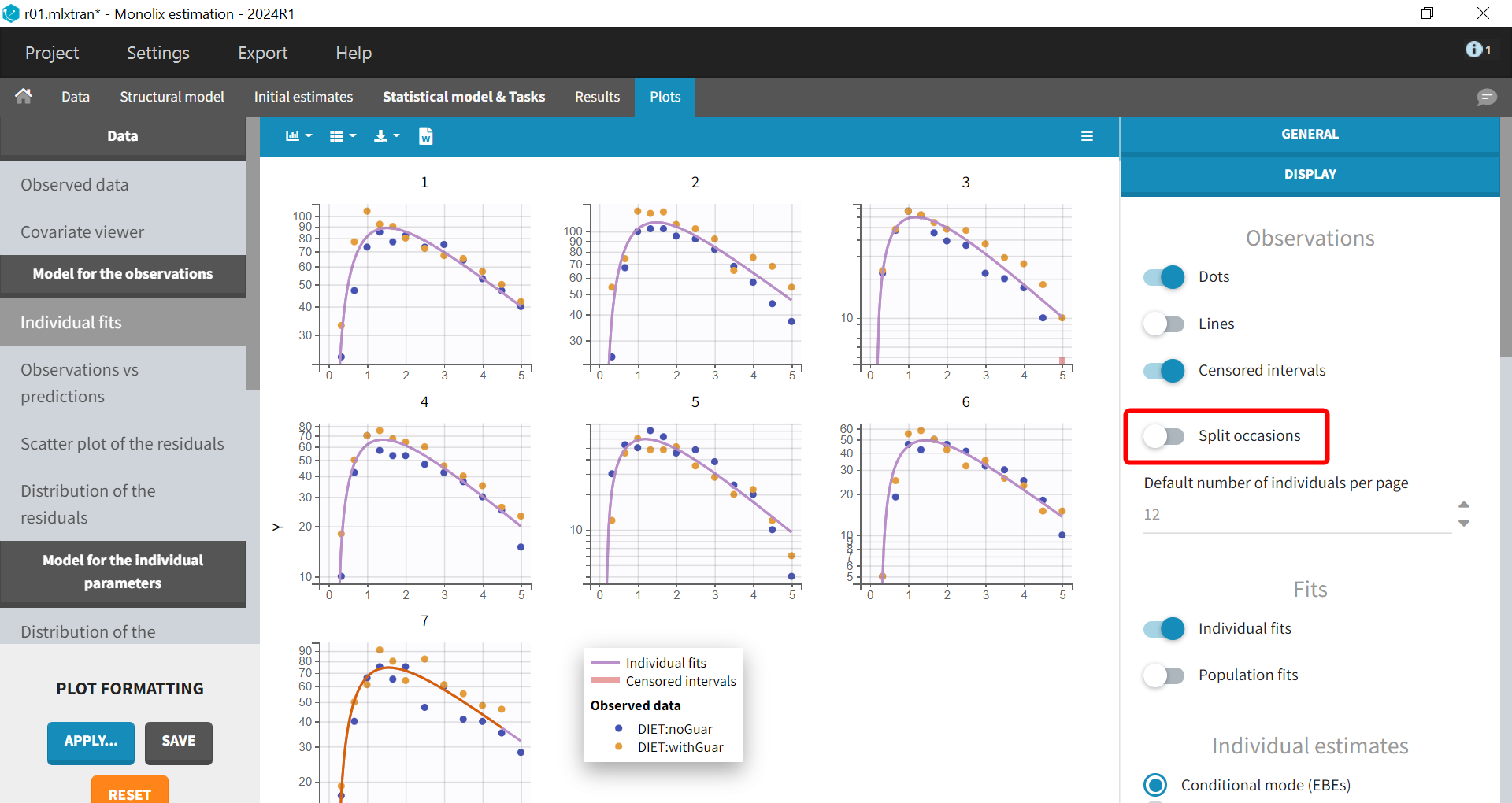
In this case, the predictions are identical for both occasions and overlap, since no inter-occasion variability is taken into account in the model. The prediction curves are displayed in purple for the first occasion and orange for the second, by default the curve for the first occasion on top, except for the last individual for which the second occasion is on top because it corresponds to a shorter observation period.
The individual fits shows that capturing both occasions with the same prediction is not possible, because there are small non-random variations from one occasion to another, as seen during the data exploration. This could corresponds to variability in the parameters between the occasions, that could be captured in the “Statistical model & Tasks” tab, by adding some random effects at the inter-occasion level or defining a covariate effect of DIET. The initial focus will be on incorporating random effects.
Model with relative bioavailability and unexplained inter-occasion variability
Each parameter can be modelled with IIV, IOV or both. Physiological considerations can help deciding if a parameter should have variability at each level or not. But in the absence of clear physiological knowledge, a possible approach is also to add a random effect at the occasion level on each parameter for which variability may be relevant, and check if the estimated standard deviation of the random effect is small.
In this scenario, all parameters exhibit potential inter-occasion variability. Elimination may vary across different periods, and the addition of guar gum could influence the absorption parameters Tlag and ka. While the volume V is less likely to fluctuate significantly between occasions, in this case, V represents the apparent volume, which also includes alcohol bioavailability that may be affected by guar gum. Therefore, a random effect for IOV could be applied to V, or alternatively, the structural model can be adjusted to explicitly account for bioavailability, allowing the random effect to be placed on bioavailability rather than volume. This approach will be implemented.
Before modifying the structural model, the most recent estimates are used as new initial values to facilitate estimation in the next run.
Next, the structural model is opened in the editor, and the add an argument p=F to the pkmodel macro. This means that the proportion of the absorbed drug will be determined by the parameter F, which should also be added to the input list:
[LONGITUDINAL]
input = {Tlag, ka, V, k, F}

EQUATION:
; PK model definition
Cc = pkmodel(Tlag, ka, V, k, p=F)

OUTPUT:
output = Cc
The “check syntax“ button is convenient to check that there is no syntax error. The modified model is then saved under a new name.
The new model can then be loaded in Monolix instead of the previous one.
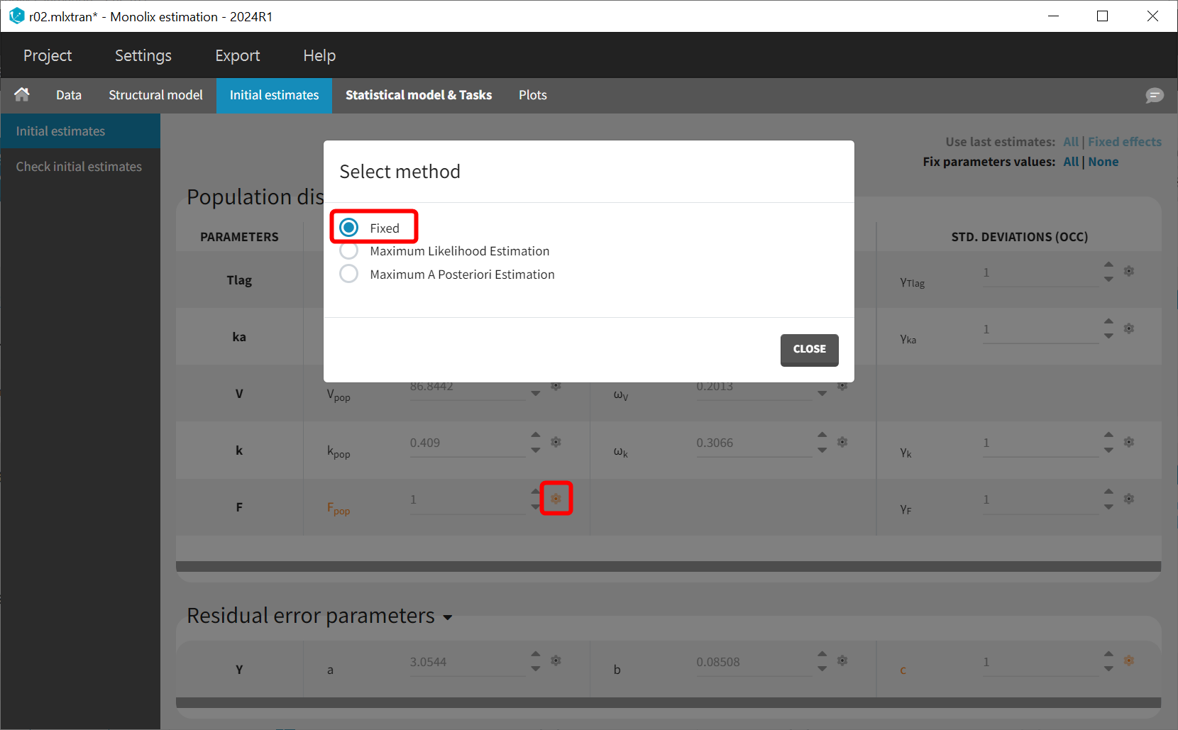
After loading the model, Monolix brings us to the “Check initial estimates” tab to choose a good initial value for F_pop. Here F is not the absolute bioavailability, but it corresponds to a relative bioavailability between the individuals. Thus F_pop is the reference value for the bioavailability, and it should be fixed to 1. This can be done in the list of the initial estimates, by changing the estimation method for F_pop to “Fixed”:
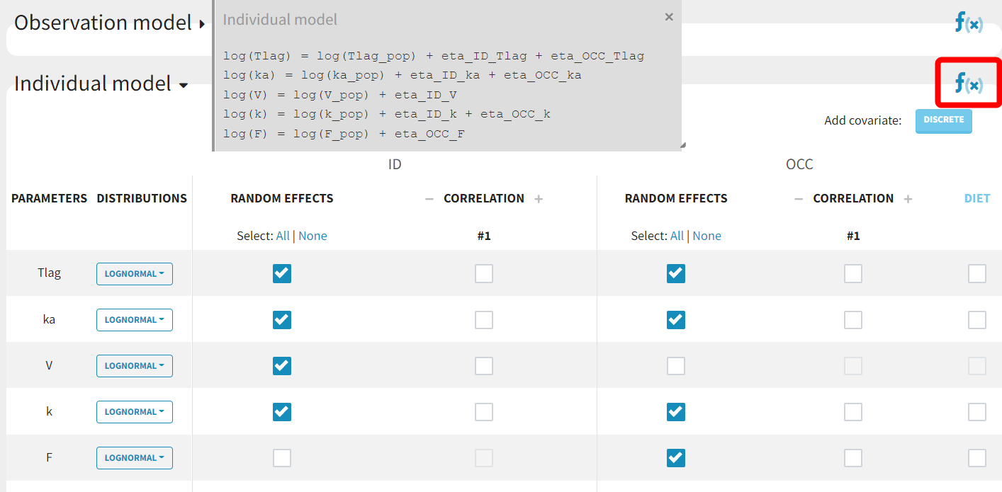
With the relative bioavailability now explicitly included in the model, inter-occasion variability (IOV) can be considered for F instead of V. Since V and F are not identifiable simultaneously, individual variability (IIV) should not be applied to F when IIV is already present for V.
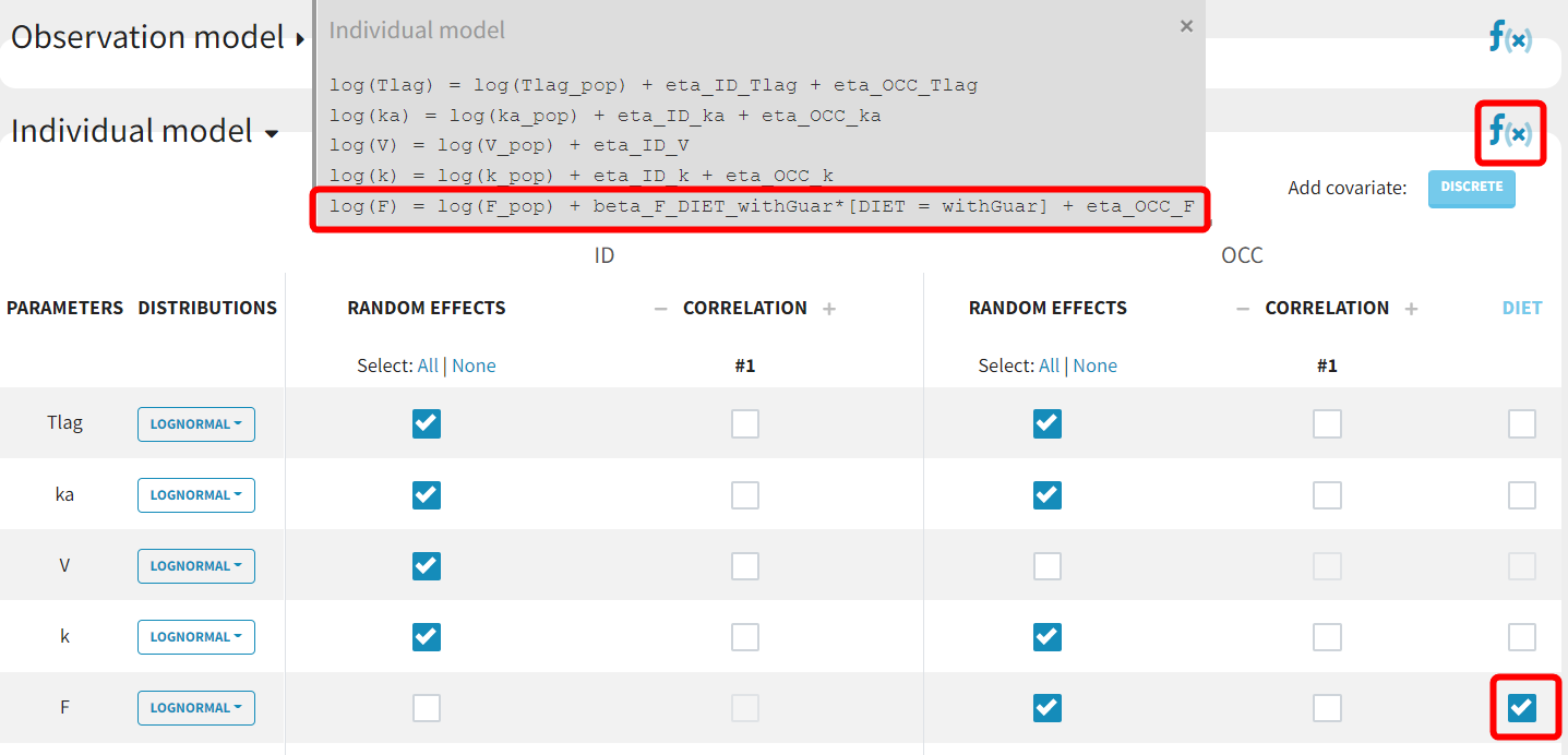
By clicking on the "f(x)" symbol the model for individual parameters is displayed. For example, the model for Tlag now includes a random effect eta_OCC_Tlag alongside eta_ID_Tlag:
This project is saved as run02.mlxtran and all tasks are run.
The table of population parameters now include the standard deviations of the new random effects at the OCC level, which are called gamma:
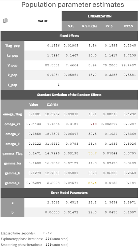
Several random effects exhibit high relative standard errors (RSEs) due to the limited size of the dataset, making it challenging to identify all random effects accurately. Random effects with the smallest standard deviations, such as omega_ka or gamma_F, could likely be removed. A more detailed assessment of which random effects to eliminate will be conducted later. For now, the focus is on examining the relationships between the random effects and the covariate DIET.
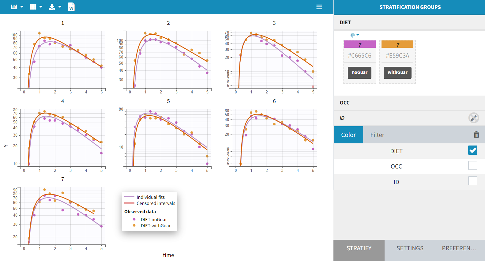
The individual fits now show different predictions for each occasion. The color scheme for the observed values, based on DIET, can be adjusted in the "Stratify" section to align with the predictions. Predictions from occasion 1, associated with the noGuar category, are displayed in purple, while those from occasion 2, linked to withGuar, are shown in orange.
fter enabling the "Information" toggle, the individual parameter values appear on the plots for each occasion (for example here for the two first individuals):
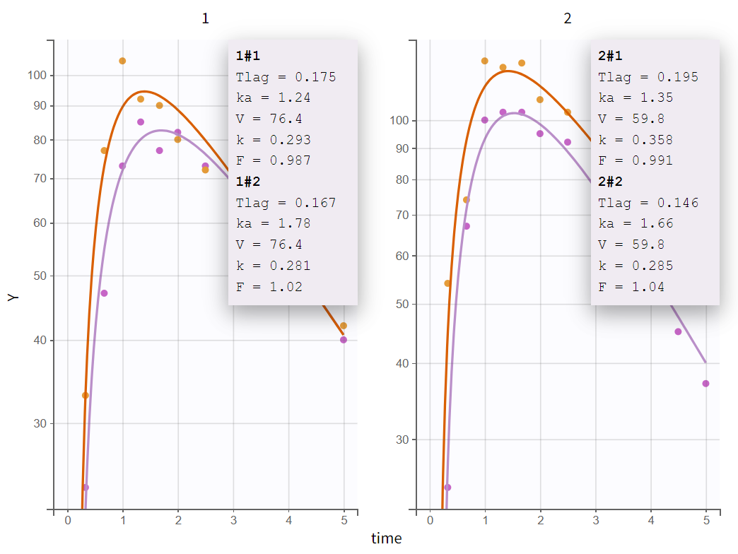
For V, which has only IIV, a single value is estimated for each individual across both occasions. For F, which has only IOV, it is important to note that estimated individual random effects from the distribution defined by gamma_F are independent across ids and occasions, and take into account the fact that F is slightly different for all subject-occasions. So a different value is estimated for each subject-occasion. Thus, the inter-occasion variability represents also an inter-individual variability. For parameters that have both IIV and IOV (Tlag, ka and k), the variability at the id level represents the additional variability between individuals that is common across both occasions.
The individual fits show that the IOV allows to properly capture the observations for each subject-occasion, and the predicted alcohol concentration seems usually higher when individuals have taken guar gum, except for ids 5. Let’s check this with the other diagnostic plots.
Assessing the effect of guar gum on alcohol’s PK
First, the plot of individual parameters vs covariates can be used to compare the distributions of each parameter across the two occasions.
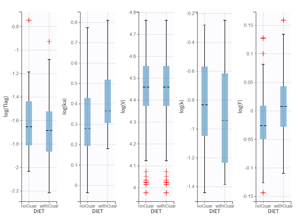
Visible differences are observed in the parameters ka, k, and F. Kinetics with guar gum show higher absorption rates and bioavailability, along with lower elimination rates. To account for these differences, a covariate effect could be implemented in the model, initially hypothesizing that guar gum impacts alcohol bioavailability.
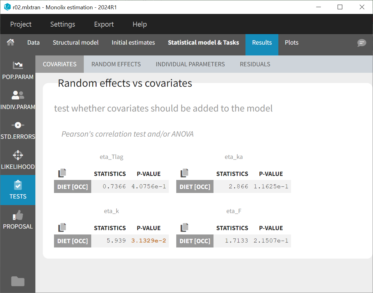
Statistical tests in the Results show no significant correlation between eta_ka and DIET. A borderline significant correlation with eta_k is observed, while eta_F shows the second lowest p-value, though it is neither significant nor borderline. The lack of significance for ka and F is likely due to the small dataset size, which impacts the p-values.
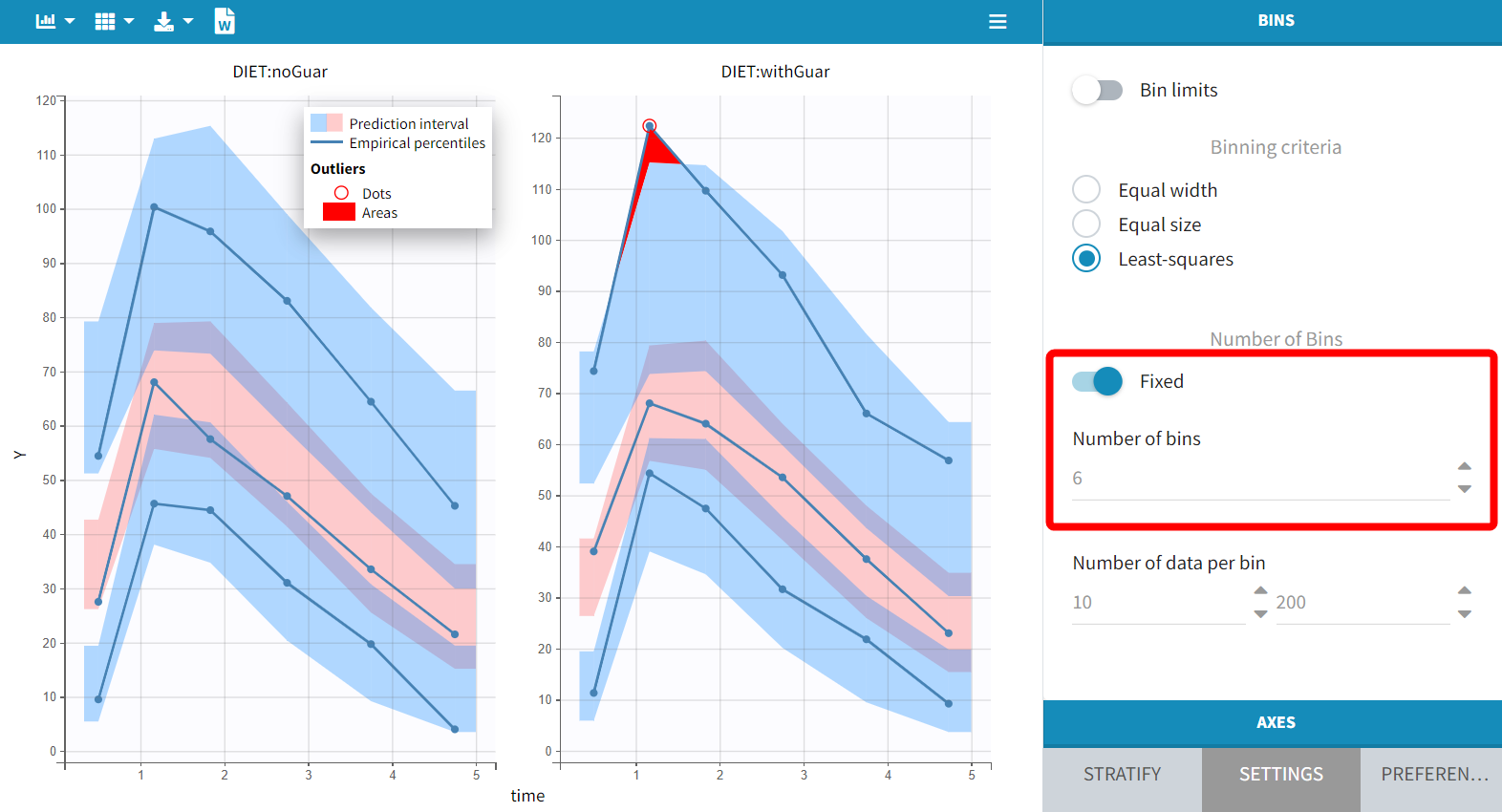
Next, examine the VPC split by DIET. The prediction intervals, derived from simulations using the IOV included in the model, remain consistent across plots, as IOV is independent of DIET. Consequently, while the prediction intervals are nearly identical for each plot, the empirical curves vary according to DIET.
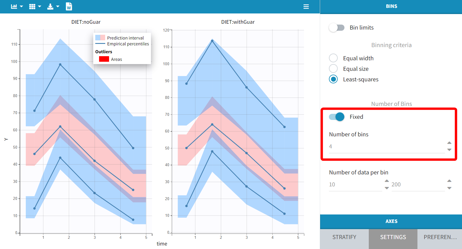
With the default setting of 4 bins, the empirical curves align well with the prediction intervals, indicating that small differences due to guar gum are not significantly affecting the model with this data size. However, increasing the number of bins to 6 reveals a minor discrepancy during the absorption phase. While the empirical percentiles are based on a limited number of individuals, this observation suggests that considering the impact of guar gum on absorption or bioavailability may be relevant.
Model with inter-occasion variability and occasion-varying covariate effect
Following this diagnosis, the model will be adjusted using the latest estimates as new initial values. Based on diagnostic plots and the understanding of guar gum's potential effects, a covariate effect of DIET on F will be added to account for part of the inter-occasion variability. The modified project is saved as run03.mlxtran, and all tasks are executed.
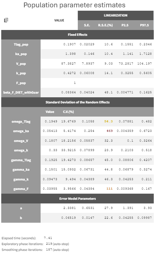
The new parameter beta_F_DIET_withGuar is estimated to a small value (0.08)but with a moderately increased standard error", and it results in a small decrease of gamma_F (from 0.05 to 0.039):
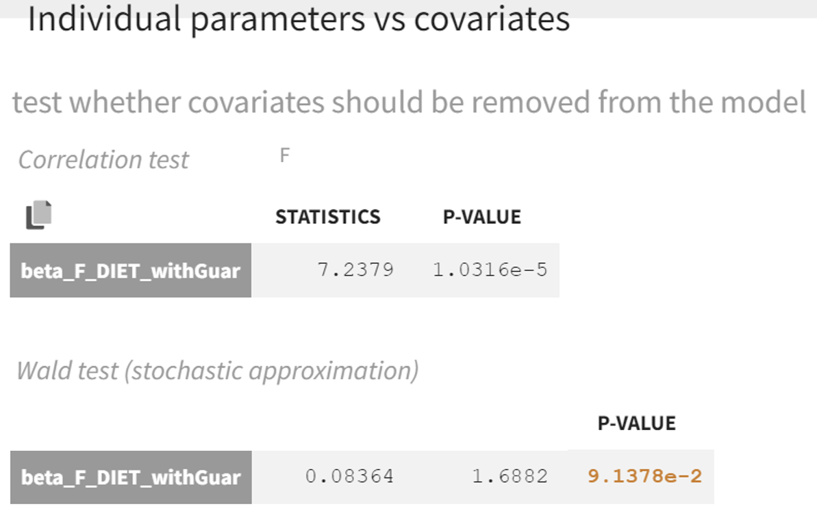
In the statistical tests, the p-value for the Wald test, which checks whether the parameter is close to 0, is small but the test is not quite significant. In addition, the correlation between F and DIET is significant:
The diagnostic plot also show that this impact is strong:
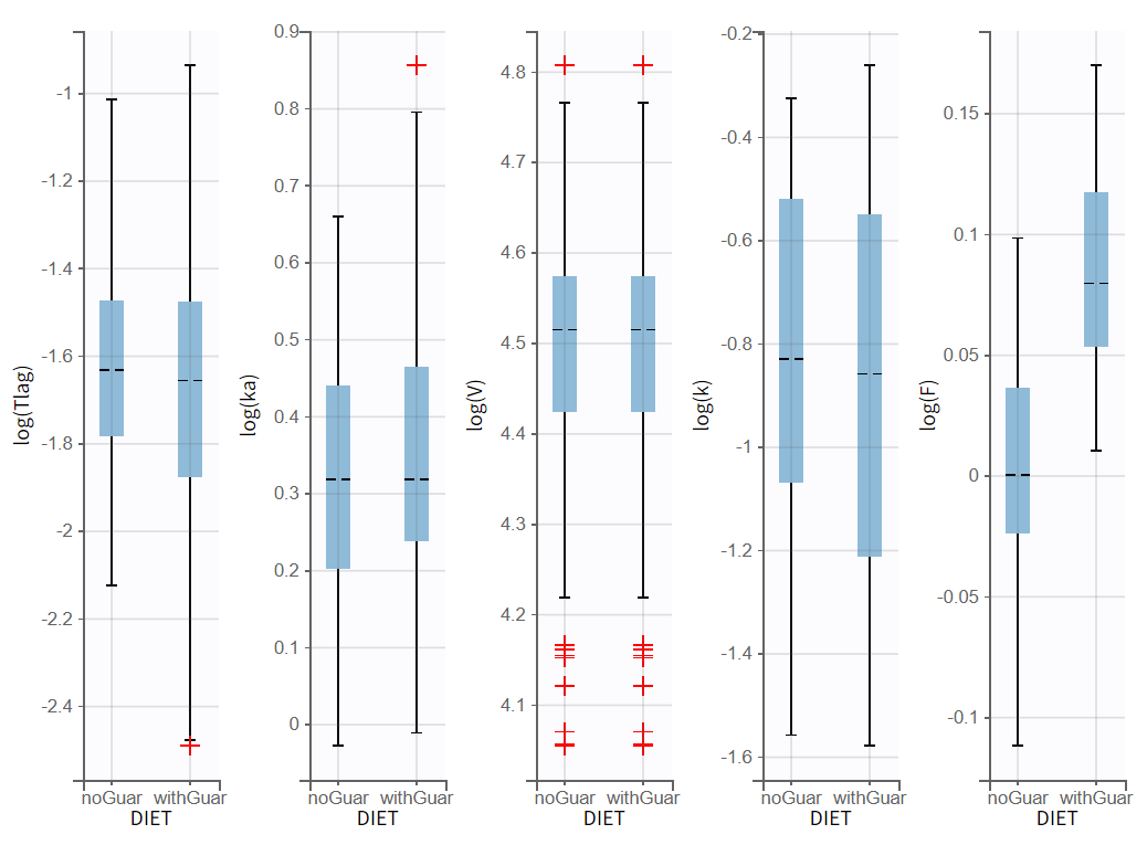
Therefore the covariate effect is relevant and should not be removed from the model.
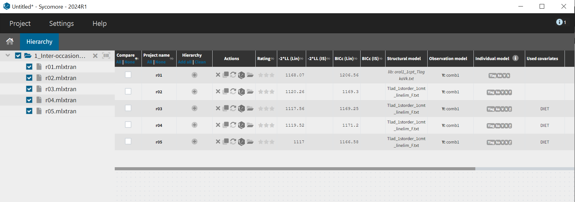
Moreover, the -2*LL for run03.mlxtran is slightly smaller than run02.mlxtran (2.7 points of difference), showing that the modified model still captures the data as well as the previous run. This can be seen easily by comparing the runs in Sycomore:
Estimation without simulated annealing
The last step involves a more detailed evaluation of whether certain random effects are poorly estimated and may need to be removed.
In the subsequent run, the settings of SAEM will be adjusted to disable simulated annealing.
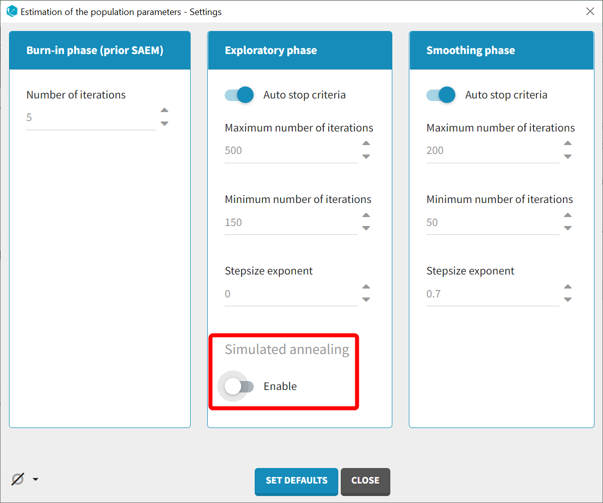
This video provides a detailed explanation of this option. Briefly, it constrains the variance of random effects to decrease gradually during estimation, which helps explore a broader parameter space and avoid getting stuck in local maxima. However, simulated annealing can also lead to artificially high omega values and hinder the identification of parameters with true zero variability, resulting in large standard errors. Therefore, when large standard errors are observed for random effects, such as omega_ka and gamma_F in this case, it is advisable to disable simulated annealing once the estimated parameters approach the solution.
Before adjusting the settings, the latest estimates should be used as initial values to ensure proximity to the solution. The modified project is saved as run04.mlxtran, and SAEM is executed. In the graphical report, omega_ka and gamma_F are observed to decrease to very small values.
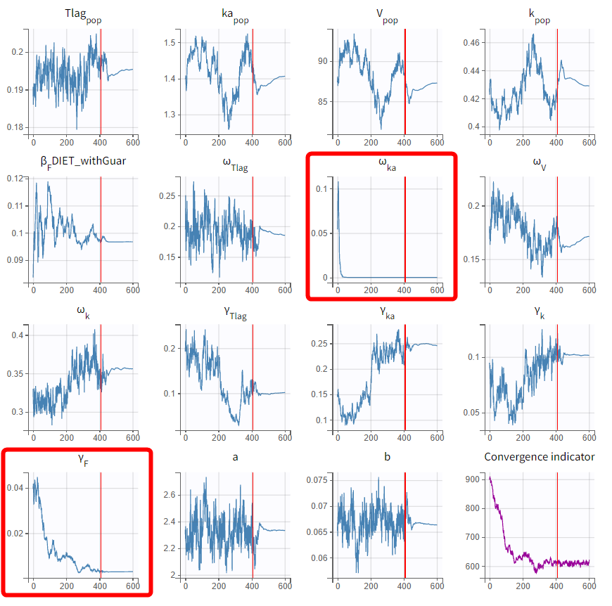
This confirms that the data does not provide sufficient information to identify the distributions for ka and F. Consequently, the last estimates should be used, and the inter-individual variability (IIV) on ka and the inter-occasion variability (IOV) on F can be removed. The IOV on F can be eliminated while retaining the covariate effect of DIET, as F also exhibits no IIV.
Following these adjustments, the entire scenario was re-run for the new project run05.mlxtran. All parameters are now estimated with relatively good standard errors, given the small size of the data.
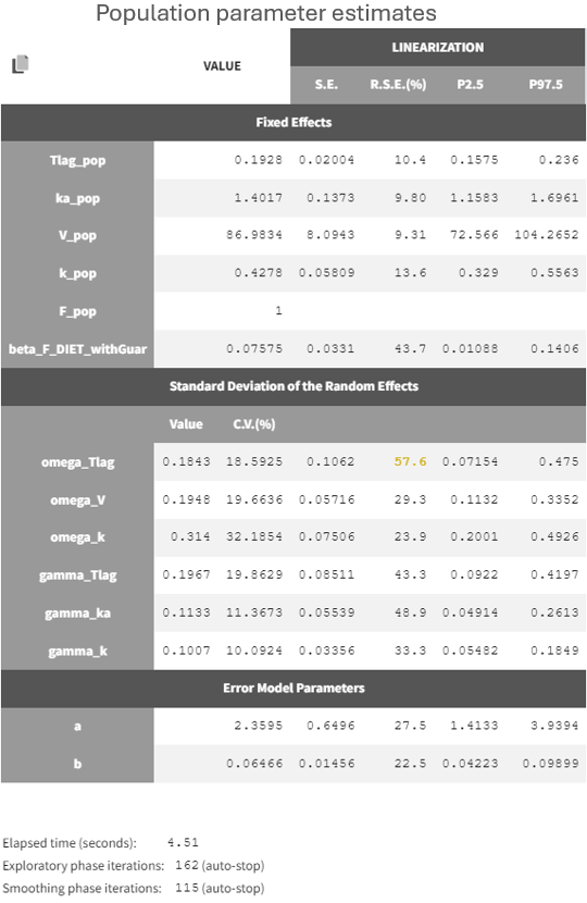
With the covariate effect on DIET on F, the discrepancy in the VPC for the occasions with guar gum is slightly smaller but still present, and is likely due to the variability in the data:
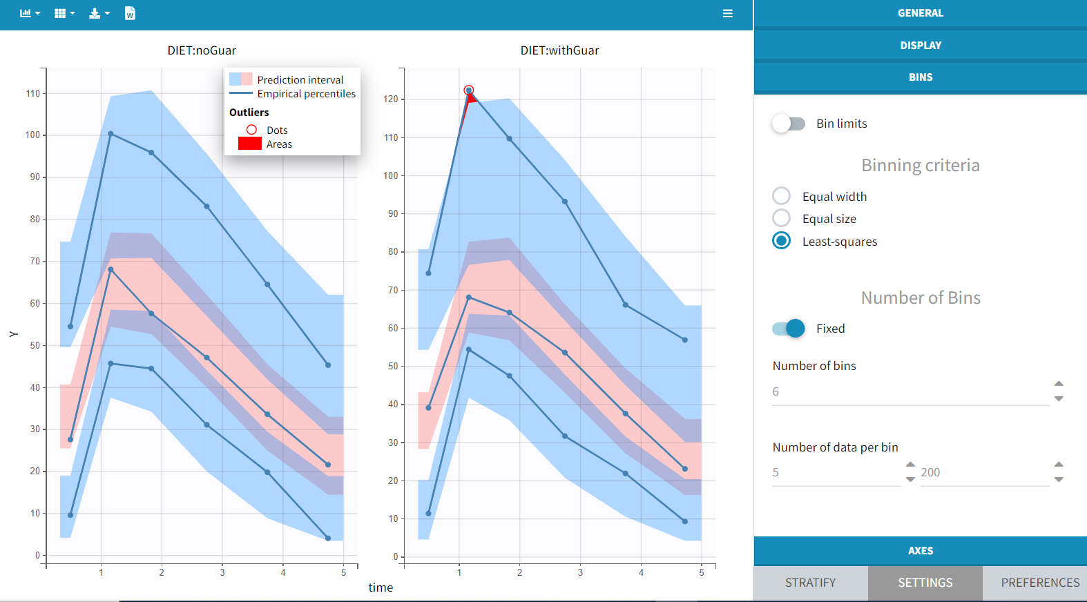
This run is the final model. Despite the small size of the data, it is able to take into account IIV and IOV, and to explain a modest part of the inter-occasion variability in bioavailability of alcohol by the effect of guar gum.

