Biosimilar Study Development - Optimizing Dose and Study Size for Pegfilgrastim

This case study documents a model-informed workflow for designing pegfilgrastim PK/PD biosimilarity studies in MonolixSuite. It summarizes the EMA/FDA biosimilar framework and uses PK/PD simulations to assess study sensitivity to plausible product differences in delivered dose, clearance, and potency. A 2x2x2 crossover clinical trial simulation evaluates the sample size needed to achieve an 80% probability of meeting standard bioequivalence criteria (90% CI within 80–125%) for PK and PD endpoints. The workflow aligns with EMA/FDA expectations for PK/PD-driven evidence generation and helps design studies that are both scientifically robust and cost-efficient.

Download Part 1 Analysis Material | Download Part 2 Analysis Material

Regulatory context

Regulators define a biosimilar as a biological product that is highly similar to an authorized reference product, allowing for minor differences that do not affect clinical performance. EMA frames the standard as demonstrating similarity in quality, biological activity, safety, and efficacy, while FDA frames it as no clinically meaningful differences in safety, purity, and potency.

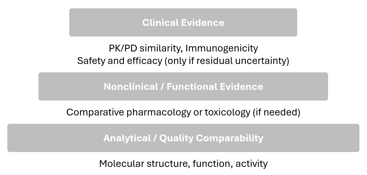
Both agencies describe a stepwise evidence-generation process that begins with comparative analytics and proceeds to targeted nonclinical/clinical studies as needed to reduce residual uncertainty.

The final determination is made through an integrated assessment (EMA “comparability exercise”; FDA “totality of evidence”).

FDA guidance positions clinical pharmacology as a key component for the biosimilarity demonstration that builds on comparative analytical evidence and can inform the need for additional clinical studies. Similarity assessments commonly use an average bioequivalence approach with a 90% confidence interval for exposure measures; 80–125% is referenced as a typical starting range in FDA’s clinical pharmacology guidance, and EMA’s bioequivalence guideline specifies reporting the point estimate and 90% confidence interval for the ratio of the test and reference product for PK parameters.

FDA notes that modeling and simulation can support dose selection for PK/PD similarity studies, particularly when PD biomarkers are used, by selecting conditions that are sensitive to detecting differences (e.g., avoiding plateau regions). This motivates this case studie’s dose-sensitivity simulations prior to power/sample size evaluation.

Consistent with the stepwise approach, the need for a comparative efficacy study depends on how much uncertainty remains after comparative analytical and PK/PD evidence. FDA’s October 2025 draft guidance notes that comparative analytical assessment (CAA) is generally more sensitive than a comparative efficacy study for detecting product differences.

Pegfilgrastim case study

Pegfilgrastim (reference product: Neulasta) is a PEGylated recombinant human granulocyte colony-stimulating factor (G-CSF) used in oncology supportive care. Its primary clinical role is prevention and shortening of chemotherapy-induced neutropenia, a dangerous reduction in neutrophils that increases infection risk and can lead to chemotherapy dose reductions or delays. By stimulating neutrophil production in the bone marrow, pegfilgrastim supports faster recovery between chemotherapy cycles and can reduce neutropenia-related complications and hospitalizations.

Pegfilgrastim is target for biosimilar development because it is widely used and biosimilars can reduce treatment costs and improve access, while still requiring a rigorous demonstration of similarity due to the inherent complexity and manufacturing sensitivity of biologics.

Mechanism of action

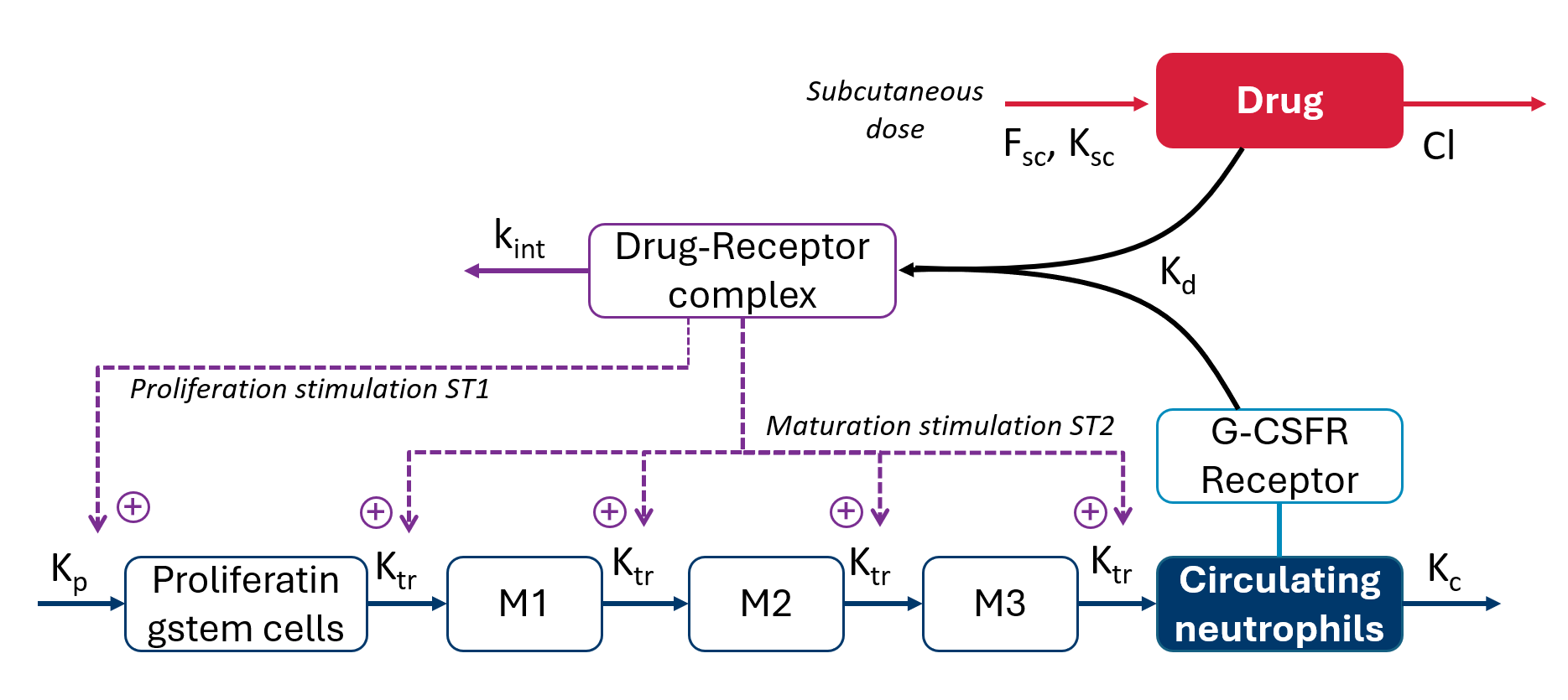
The drug exerts its effect by binding to the G-CSF receptor (G-CSFR) and stimulating neutrophil production and maturation, leading to an increase in circulating neutrophils. In clinical pharmacology studies and in this case study, the pharmacodynamic (PD) response is captured using absolute neutrophil count (ANC).

A key characteristic of pegfilgrastim is that effect and clearance are coupled. As ANC increases, the extent of receptor-mediated elimination can increase because more neutrophils provide more receptor capacity, reinforcing a feedback loop: drug exposure drives ANC upward, and higher ANC can accelerate elimination. This interaction contributes to nonlinear pharmacokinetics and is commonly described as target-mediated drug disposition (TMDD).

Scientific basis and model selection

Two published modeling-and-simulation analyses provide the inpiration for this case study and motivate both the PK/PD model choice and the sensitivity factors explored for dose and design decisions.

Li et al. (2022): Adapted a previously published semimechanistic PK/PD model to better represent healthy-subject pegfilgrastim data, verified it across the 2–6 mg range, and then performed structured sensitivity simulations to quantify how PK/PD similarity endpoints respond to

• small delivered dose-amount changes and

• changes in clearance mechanisms specifically linear clearance (CL-linear) and

• receptor binding affinity (Kd, linked to nonlinear/TMDD clearance)

using AUC/Cmax and ANC-based endpoints (AUEC/ANCmax).

Brekkan et al. (2019): Used simulations from a previously developed population PK/PD model to evaluate how plausible “product differences” translate into PK/PD similarity outcomes and study power in a typical phase I setting. The model used in Brekkan et al. differs from the Li et al. framework in its level of mechanistic detail.
Using this setup, Brekkan et al. simulated a two-way crossover similarity study in healthy volunteers (nominally 6 mg s.c.) and tested scenarios with differences in

• delivered (bioavailable) dose amount,

• potency (implemented as EC50 changes), and

• baseline ANC

PK/PD similarity was summarized using AUC and AUEC(ANC), and statistical power to conclude similarity was computed under varying sample sizes.

Building on these studies, the sensitivity analyses for dose selection and subsequent study design optimization are conducted using the Li et al. model (a mechanistic TMDD model with a quasi-equilibrium assumption), rather than the Brekkan et al. model (a more simplified TMDD representation using Michaelis–Menten kinetics), because Li et al. explicitly adapted and verified the model for healthy subjects across 2–6 mg, enabling dose-to-dose sensitivity comparisons on the intended range.

Model source: Li et al. (2022) (doi:10.1002/cpt.2722)
Supporting Information: cpt2722-sup-0001-supinfo.zip (download from the journal article page)

Model

The conduct of the case study in MonolixSuite required a re-implementation. The model has been translated from NONMEM to mlxtran.

Structural model

The translated structural model looks as follows:

[LONGITUDINAL]
input = {ksc, Fsc, V, Cl, kp, ktr, kc, Kd, kint, STM1, STM2, SR, bsld}

PK:
depot(target = A2, ka = ksc, p = Fsc * 1e6 / 18800)

EQUATION:
; conversion
ke = Cl/V

; ----------------------------------------
; PK initial conditions
t_0  = 0
A2_0 = 0

; PK equation system
;ddt_A1 = -ksc*A1
TD = A2/V
TR = A7
FD = 0.5*((TD-TR-Kd)+sqrt((TD-TR-Kd)^2+4*Kd*TD))
RD = TD - FD

ddt_A2 =  - ke*FD*V-kint*RD*V
CONC = FD + bsld

;-----------------------------------------
; PD initial conditions
A3_0 = kp/ktr   
A4_0 = kp/ktr   
A5_0 = kp/ktr  
A6_0 = kp/ktr 
A7_0 = kp/kc 

;PD equation system
ST1 = 1 + STM1*(RD/TR)
ST2 = 1 + STM2*(RD/TR)
ddt_A3 = kp*ST1-(ktr*ST2)*A3
ddt_A4 = ktr*ST2*A3 - ktr*ST2*A4
ddt_A5 = ktr*ST2*A4 - ktr*ST2*A5
ddt_A6 = ktr*ST2*A5 - ktr*ST2*A6
ddt_A7 = ktr*ST2*A6 - kc*A7
ANC = A7/SR

OUTPUT:
output = {CONC, ANC}

Unit conversion

The published model is defined on a molar concentration scale: PK concentrations are in nM (nmol/L) (e.g. Kd in nM and the baseline term bsld in nM), and the key PD-driving parameters are also nM-based (e.g.,kp in nM/h). This implementation keeps the internal units unchanged.

The only unit-related adjustment is at dose input, where the depot amount is scaled by to convert doses entered in mg to nmol (using MW = 18,800 g/mol). This input conversion is used to run simulations at clinically stated doses (2, 4, 6 mg) while preserving the original molar-scale parameterization. With A2 in nmol and V in L, TD=A2/V remains nmol/L (nM), so FD and CONC=FD+bsld stay in nM.

Statistical model

The published statistical model includes IIV terms and covariances between random effects and specifies an exponential residual error model for PK and PD. In MonolixSuite, the same statistical assumptions and parameter estimates are used. Covariance terms reported in the publication are converted to correlations.

The residual error is implemented as a constant error model under a lognormal distribution, which is equivalent to an exponential error model.

Part 1: Dose selection

The dose-selection step evaluates which dose (2, 4, 6 mg) provides the highest sensitivity to detect plausible product-related differences by comparing simulated changes in PK exposure (AUC, Cmax) and PD metrics (AUEC(ANC), ANCmax) under controlled perturbations of delivered dose, potency/binding (Kd), and clearance (CL-linear). Using the published pegfilgrastim PK/PD model, the workflow simulates one (the same) typical healthy subject across all three dose groups and applies one parameter change at a time to isolate the impact of each potential source of product-related variability.

• Delivered-dose differences are represented via Fsc changes from −10% to +10% in 2% increments, while

• potency (Kd) and linear clearance (CL-linear) are each varied separately from −50% to +50% in 10% steps.

Endpoints are then summarized as ratios versus the unperturbed baseline (0% change) to enable a direct, dose-by-dose comparison of sensitivity across perturbations.

Simulation setup

The simulations are conducted in Simulx in which the core simulation elements (model + population parameters, covariates, treatments, and outputs) are defined in the project definition. The underlying model structure and population parameter estimates are taken from the literature model described earlier (Link to Li et al 2022)

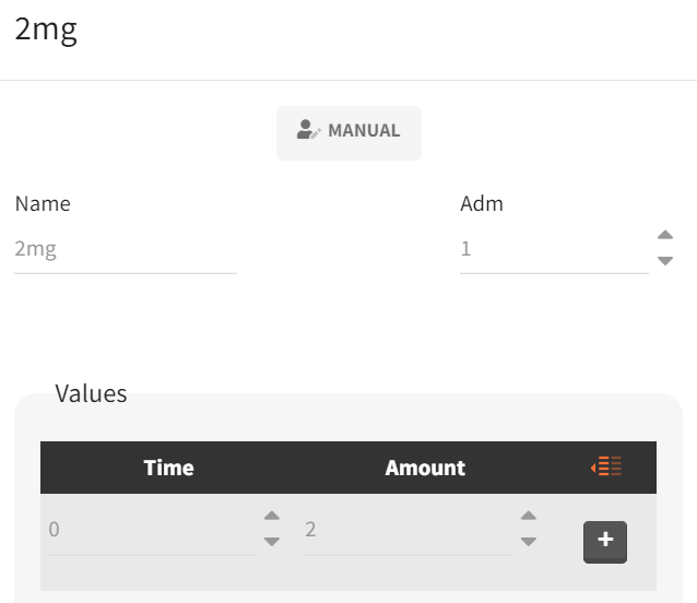
Because simulations are performed across three dose groups, separate treatment elements are defined for each regimen. In the “Definition” tab (sub-tab “Treatment”), a new treatment element is created for each dose with a clear name (e.g., 2mg, 4mg, 6mg) and a single subcutaneous administration at time 0, using the corresponding amount (2, 4, or 6 mg). The same procedure is repeated for the other treatments.

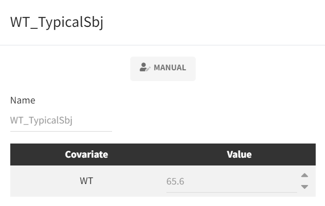
Because the analysis is intended to represent a typical subject and the model includes a body-weight covariate effect, a covariate element is defined in the subtab “Covariates“ to fix body weight to the literature “typical” value (65.6 kg) used for the simulations.

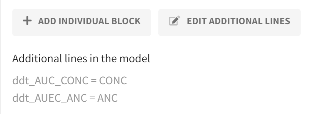
Before defining output vectors, the model is extended to calculate cumulative exposure/effect metrics directly during simulation. This is implemented in the “Definition“ tab in the “Model“ subtab via the Additional lines feature by adding two equations that integrate the concentration and ANC profiles over time (i.e., a running integral). Solving these equations yields AUC(CONC) and AUEC(ANC) as additional model outputs.

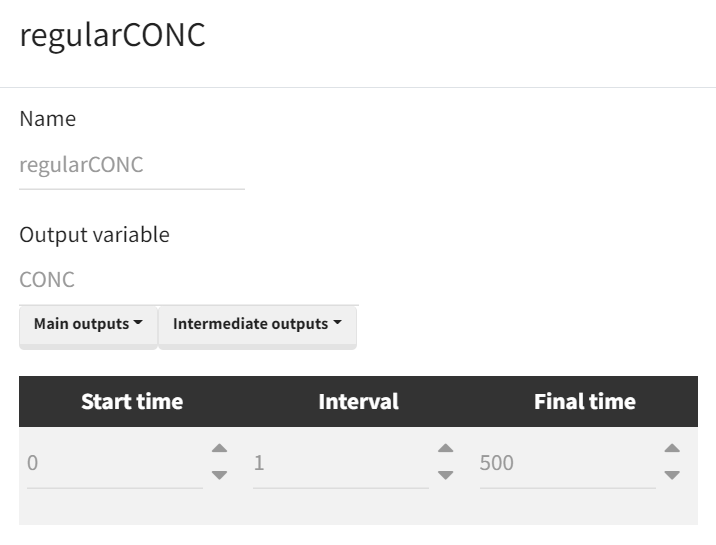
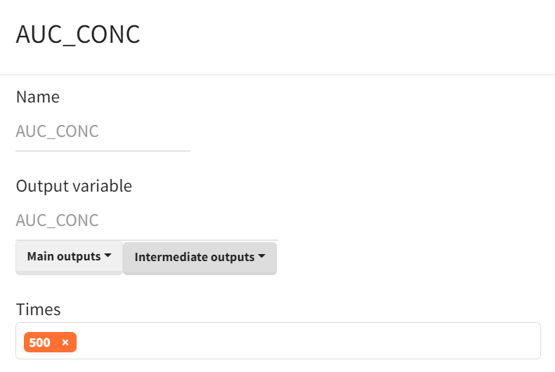
Output vectors required for the analysis are then defined in the “Definition” tab (sub-tab “Output”) and include the full CONC–time and ANC–time profiles. For visualization and to ensure that concentrations/effects have returned close to baseline before computing cumulative metrics, the output horizon is extended to time 500. The cumulative AUC/AUEC outputs are retained as vectors internally, and the final value at time 500 is used as the scalar AUC(CONC) and AUEC(ANC) for endpoint extraction.

Time curve	Area under the curve

Note: output definition is done analoguously for ANC and AUEC.

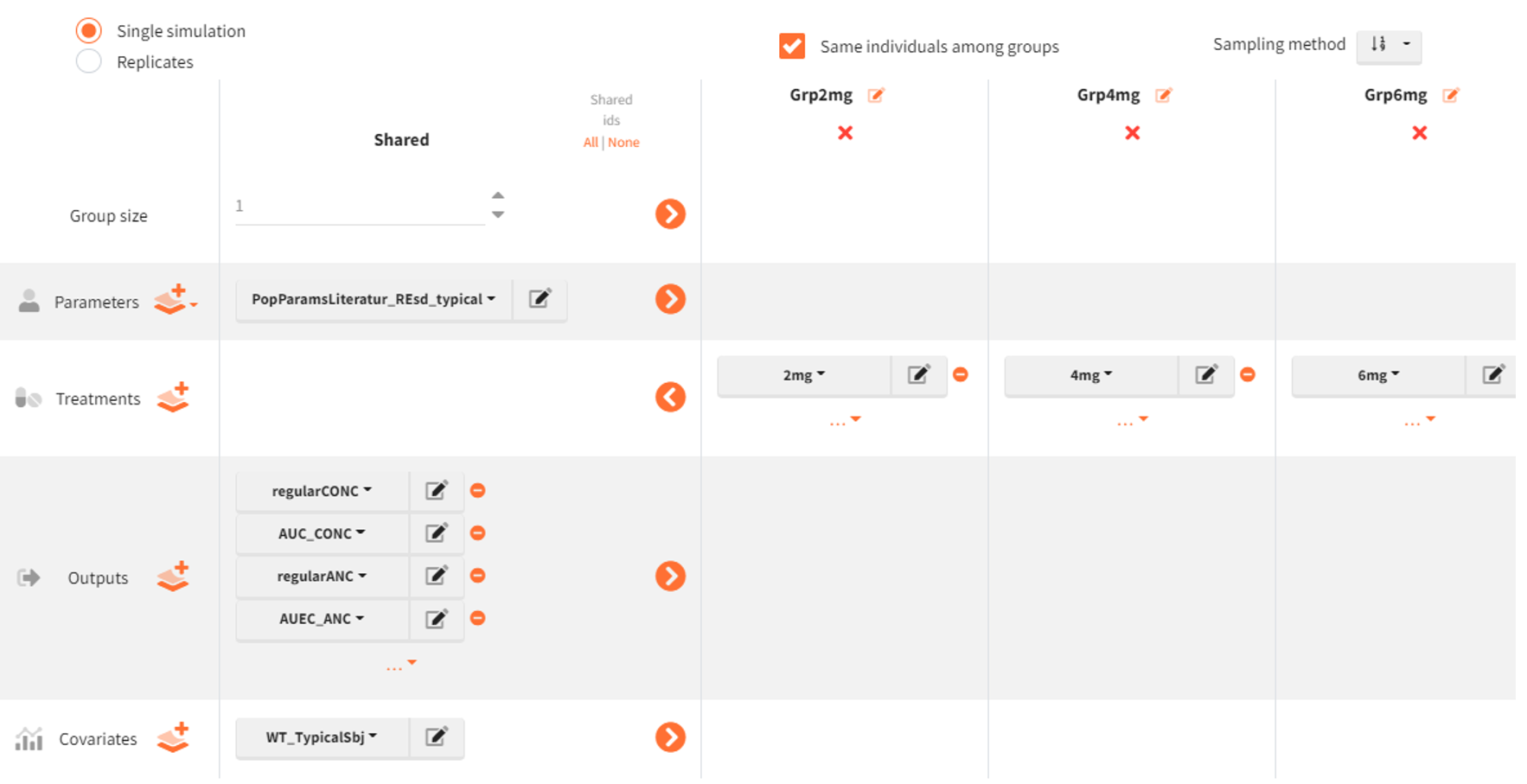
The simulation scenario is defined as follows:

• The population parameter element is set to PopParamsLiteratur_REsd_typical, populated with literature estimates, with omega (IIV) parameters set to 0.

• Three simulation groups are created: Grp2mg, Grp4mg, and Grp6mg, differing only by the treatment elements 2mg, 4mg, and 6mg.

• The following output vectors are selected for simulation: regularCONC, AUC_CONC, regularANC, AUEC_ANC.

• The covariate element WT_TypicalSbj is used to fix body weight to the typical-subject value.

• Group size is set to 1 for each simulation group.

• The option “Same individuals among groups” ensures the same subject is represented across all dose groups. In our case, in the absence of random effects (omegas set to zero), this option has no effect but we select it for clarity.

Post-processing: outcomes and endpoints

For the sensitivity analysis, the simulation outputs require post-processing to derive the final comparison metrics. This post-processing is configured in Simulx using the Outcomes & Endpoints module. Part of the required metrics is already produced during simulation via the outputs namely AUC(CONC) for the concentration time profile and AUEC(ANC) for the ANC time profile. The remaining metrics Cmax and ANCmax are defined as outcomes in the “Outcomes & Endpoints” module; in the same step, AUC and AUEC are also defined as outcomes/endpoints so that all four metrics are available in one place and returned in a consistent format.

Peak of time curve	Area under the curve

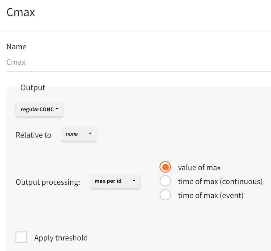
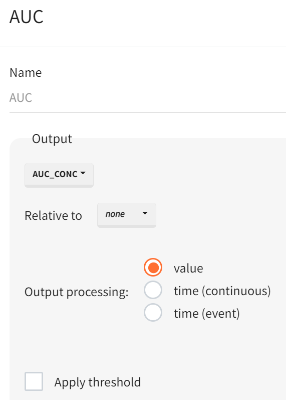
Definitions for ANCmax and AUEC follow the same logic. Simulx automatically creates corresponding endpoints when outcomes are defined. In this typical-subject setup (one simulated individual per group), the endpoint setting (e.g., arithmetic mean, geometric mean, median) is not material because each simulation group produces a single value; however, the configuration still requires explicit definitions of all four outcomes (Cmax, AUC, ANCmax, AUEC) and therefore results in four endpoints.

This setup does not yet include any parameter perturbations. It serves as the base template Simulx project that is loaded for each iteration in the parameter-scenario sweep.

Automated parameter perturbation

To avoid creating a separate Simulx project for every parameter-change scenario, the sensitivity workflow is automated in R with LixoftConnectors. The scenario grid includes delivered-dose perturbations implemented through Fsc from −10% to +10% in 2% steps (11 scenarios), and potency (Kd) and linear clearance (CL) perturbations from −50% to +50% in 10% steps (11 scenarios each). Each scenario requires updating a single parameter (one-at-a-time), followed by simulations and endpoint extraction across the three dose groups (2, 4, 6 mg). Without automation, this corresponds to 33 scenario runs that would otherwise need to be configured and executed manually.

rm(list = ls())
path.prog <- dirname(rstudioapi::getSourceEditorContext()$path)
library(dplyr)
path.software <- paste0("C:/Program Files/Lixoft/MonolixSuite2024R1")
library(lixoftConnectors)
################################################################################
initializeLixoftConnectors(path.software, software = "simulx")
project <- paste0(path.prog, "/s01_TypSbj_PreRun_Template.smlx")
loadProject(project)

# Define individual change sets for parameter pertubations
fold_Fsc   <- seq(-0.1, 0.1, by = 0.02)
fold_kdCl  <- seq(-0.5, 0.5, by = 0.1)

# Combine parameter pertubations into scenario table
scenarios <- bind_rows(data.frame(param = "Fsc_pop", fold = fold_Fsc),
                       data.frame(param = "kd_pop",  fold = fold_kdCl),
                       data.frame(param = "Cl_pop",  fold = fold_kdCl)) 

nb_sen <- length(scenarios[,1])
# Retrieve original population parameter vector
popParam_base <- data.frame(getPopulationElements()$PopParamsLiteratur_REsd_typical$data)
# Result container
results_all   <- data.frame() 
#------------------------------------------------------------------------------
# Loop through parameter pertubation scenarios
for (i in 1:nb_sen) { 
  param  <- scenarios$param[i]
  fold   <- scenarios$fold[i]
  if(i>1){
    initializeLixoftConnectors(path.software,software = "simulx")
    loadProject(project)
  }
  popParam_mod <- popParam_base %>%
    mutate(!!as.character(param) := .data[[as.character(param)]] * (1+fold))

  scenario_name <- paste0(param, "_", fold*100, "percfold")
  popElem_name <- paste0("PopParams_", scenario_name) %>%
    gsub("-", "m", ., fixed = TRUE) %>% 
    gsub("\\+", "p", .)   
  
  definePopulationElement(name=popElem_name, element = popParam_mod)

  setGroupElement(group = "Grp2mg", elements = c(popElem_name))
  setGroupElement(group = "Grp4mg", elements = c(popElem_name))
  setGroupElement(group = "Grp6mg", elements = c(popElem_name)) 

  setSameIndividualsAmongGroups(TRUE) 
  # set calculation of both simulation and endpoints
  setScenario(c(simulation = T, endpoints = T))
  # printSimulationSetup()
  runScenario()
  # saveProject(paste0(path.prog,"/s01_TypSbj_PostRun_",scenario_name,".smlx"))
  
  # retrieve exposures/responses from simulation endpoint results, and add additional columns
  endpnt_tmp  <- getEndpointsResults()$endpoints
  Cmaxres_i   <- data.frame(endpnt_tmp$Cmax_value) %>% mutate(Scenario = scenario_name, FoldChange = paste0(fold*100,"%"), Parameter = param, Metric = "Cmax") %>% rename(Value= geometricMean)
  AUCres_i    <- data.frame(endpnt_tmp$AUC_value)  %>% mutate(Scenario = scenario_name, FoldChange = paste0(fold*100,"%"), Parameter = param, Metric = "AUC")  %>% rename(Value= geometricMean)
  ANCmaxres_i <- data.frame(endpnt_tmp$ANCmax_value) %>% mutate(Scenario = scenario_name, FoldChange = paste0(fold*100,"%"), Parameter = param, Metric = "ANCmax") %>% rename(Value= geometricMean)
  AUECres_i   <- data.frame(endpnt_tmp$AUEC_value)   %>% mutate(Scenario = scenario_name, FoldChange = paste0(fold*100,"%"), Parameter = param, Metric = "AUEC")   %>% rename(Value= geometricMean)
  # append new results 
  results_all <- bind_rows(results_all, AUCres_i, AUECres_i, Cmaxres_i, ANCmaxres_i) 
}

In each scenario, the baseline/template Simulx project is reloaded and a single parameter is modified by applying a multiplicative fold change: parameter_new = parameter_base × (1 + fold). The updated population parameter vector is passed to all three dose groups (2, 4, 6 mg), while all other simulation elements (treatments, covariates, outputs, outcomes/endpoints) remain unchanged. Simulations are run for each parameter-perturbation scenario with the predefined Outcomes & Endpoints calculations enabled, so that Cmax, AUC, ANCmax, and AUEC are returned for each dose group. The resulting metric values are then converted to a baseline-referenced sensitivity measure by computing a ratio for each scenario and metric (e.g., metric at −10% Fsc divided by the same metric at 0% change). These ratios are then plotted across perturbation levels to visualize and compare dose-dependent sensitivity.

Note: The plotting R script is provided in the accompanying case study materials.

Results

Delivered dose (Fsc) pertubations

Across delivered dose differences (Fsc, −10% to +10%), PK exposures (AUC, Cmax) shift monotonically with the delivered dose difference at all three dose levels (2, 4, 6 mg). The exposure change is more-than-proportional relative to the delivered-dose deviation (e.g., a +10% delivered dose yielding >1.10 on the normalized AUC/Cmax scale). The normalized presentation (ratio to the 0% reference) supports direct comparison across dose groups, while the 0.80–1.25 reference lines contextualize the magnitude of the shift against standard bioequivalence limits.

In contrast, PD metrics (AUEC(ANC), ANCmax) remain essentially unchanged across the full Fsc range and accross doses, indicating limited PD sensitivity to small delivered-dose deviations within the explored window.

Potency (Kd) pertubations

When varying binding affinity/potency (Kd), the 2 mg group shows the largest PK sensitivity, while the 4 and 6 mg group shows a much smaller PK response across the same deviation range. This means that at low doses the receptor-mediated binding dominates the drug elimination processes.

Despite detectable PK shifts, pronounced at 2 mg, PD metrics remain negligible/insensitive across doses, reinforcing that the ANC response is comparatively buffered in these scenarios.

Clearance (CL) pertubations

For linear clearance perturbations, the largest PK sensitivity is observed at 6 mg, with minimal sensitivity at 2 mg. The interpretation aligns with a dose-dependent balance between clearance pathways: at low dose, exposure is comparatively insensitive to linear CL changes; at higher doses, saturation of the nonlinear pathway increases the impact of linear CL variability on exposure.

As with delivered-dose and Kd perturbations, PD metrics remain stable across the explored CL range, consistent with feedback regulation in the ANC system.

Partitioning of clearance: linear vs nonlinear contribution

Dose-dependent sensitivity patterns from Part 1 (higher sensitivity to Kd at low dose vs. higher sensitivity to linear CL at high dose) can be interpreted by quantifying how total clearance is distributed between linear and nonlinear (TMDD/internalization) pathways at each dose level.

The clearance partition is computed from simulated exposure using AUC. The model’s PK output concentration is defined as: CONC(t) = FD(t) + bsld, where FD(t) is the free-drug component and bsld is an additive baseline term. Because bsld does not represent disposition-driven drug, integrating CONC(t) would add an artificial baseline-dependent area term (bsld * T). To avoid this bias, the AUC used for total clearance calculations is defined on FD(t) only, by adding this term in the model: implemented as ddt_AUC_FD = FD.

To ensure that the AUC reflects the full exposure profile, the AUC_FD output is returned at a late time point (e.g., t = 900), chosen so that the concentration–time curve has effectively returned to baseline. The rest of the Simulx simulation scenario setup otherwise matches the setup used in the preceding analyses.

Next, total clearance can be calculated from the simulation outputs by retrieving AUC_FD​ for each dosing group applying:
Before, doses need to be converted from mg to nmol:
To partition linear versus nonlinear (TMDD/internalization) contributions, the nonlinear component is obtained by:

The corresponding fractional contributions are:
and

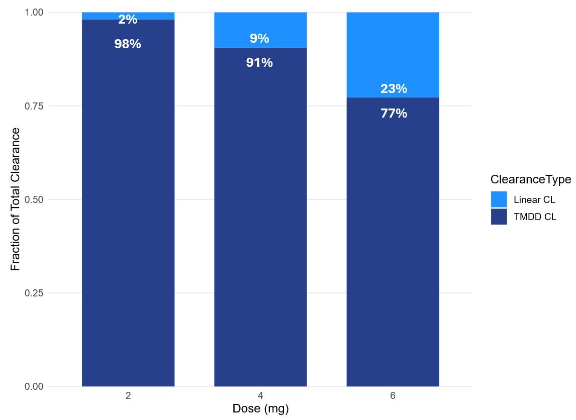
The clearance-partition plot shows a clear dose dependency in the elimination mechanisms. Based on the typical-subject simulations, the nonlinear (TMDD/internalization) pathway dominates at low dose and progressively declines as dose increases, while the linear pathway becomes increasingly relevant:

• 2 mg: TMDD 98% vs linear 2%

• 4 mg: TMDD 91% vs linear 9%

• 6 mg: TMDD 77% vs linear 23%

This pattern supports the sensitivity findings from Part 1. At 2 mg, exposure is largely governed by target-mediated elimination. As a result, Kd perturbations (which affect binding-related elimination) have greater leverage on AUC and Cmax, whereas linear CL perturbations have comparatively limited impact. At 6 mg, partial saturation of the nonlinear pathway reduces the impact of Kd changes, while the increased linear contribution makes exposure more sensitive to linear CL differences, consistent with the observed PK sensitivity ranking for CL perturbations.

Across these perturbations, PD endpoints (AUEC(ANC), ANCmax) remain largely insensitive, consistent with the feedback regulation in the ANC system dampening PD variability even when PK exposure shifts are detectable.

Note: the script for the Cl partition analysis can be found in the attached materials

Conclusion

Across delivered-dose, Kd, and CL perturbations, PK endpoints (AUC, Cmax) show clear sensitivity, while PD endpoints (AUEC(ANC), ANCmax) remain largely flat over the tested ranges. Taken together, these results support using 6 mg as the dose level for the clinical trial simulations and sample-size evaluation in Part 2, since 6 mg is the approved clinical dose for pegfilgrastim and it provides the clearest sensitivity to clearance-related exposure differences, which is the parameter which is the hardest to assess by analytical assessment.

Part 2: Study design optimization

Part 2 quantifies how likely a 2x2x2 crossover comparative PK/PD similarity study (test vs reference) is to conclude bioequivalence under realistic variability, and how that probability changes with sample size and plausible product differences. The goal is to identify the minimum sample size that still achieves the usual 80% power target for demonstrating bioequivalence (90% CI of the geometric mean ratio within 80-125%), focusing on the main sources of potential between-product differences considered in Part 1 (delivered dose, clearance, potency).

The workflow is organized around a scenario grid, replicate-trial simulation, and BE evaluation:

Define test–reference difference scenarios (applied to the test product only)

• Delivered dose (Fsc​): 0, 2, 4, 6, 8, 10%

• Linear clearance (CL) and potency (Kd): 0, 5, 10, 25, 50, 75, 100, 125, 150%

Sample size is evaluated in batches of 50 to 250 subjects (step size 50), and each scenario is defined by a specific combination of test-product perturbation (on Fsc​, CL, or Kd​) and sample-size batch.

For each scenario, 200 replicate trials are simulated. Per replicate, bioequivalence is evaluated for PK endpoints (AUC, Cmax) and PD endpoints (AUEC(ANC), ANCmax); an endpoint is considered to pass if the 90% CI of the GMR lies within 80–125%.

Power is then reported as the percentage of replicates that meet the BE criterion for each endpoint.

This analysis could be performed entirely in the Simulx GUI, but exploring multiple parameter perturbation levels, many replicate trials, and several sample-size batches would require creating and manually modifying a large number of projects, which is inefficient and increases the risk of implementation errors. Therefore, this part of the analysis is documented in two components: (1) a reusable Simulx template project, and (2) an R-based automation workflow using Lixoft connectors to generate scenarios, run replicate simulations, and summarize power.

Base Simulx project (template configuration)

Covariate - Formulation effects (R vs T) on key similarity drivers

In order to simulate a crossover trial with the reference and test product, it is necessary to encode the difference between the test and reference product in the model. To encode product-specific differences, a categorical covariate FORM is added with two categories: R (reference) and T (test). FORM drives covariate effects on the parameters used to represent potential product differences (Fsc​, CL, Kd).

FORM is declared in the model [COVARIATE] block:

[COVARIATE]
input = {WT, FORM}                                ;WT retained from the original model
FORM = {type=categorical, categories={'R', 'T'}}  ;formulation: reference (R) / test (T)

Formulation-effect coefficients are added as inputs in [INDIVIDUAL], and FORM is available for use in the parameter definitions:

[INDIVIDUAL]
input = {...,                                 
         Fsc_pop, omega_Fsc, beta_Fsc_FORM_T,
         Cl_pop,  omega_Cl,  beta_Cl_FORM_T,
         Kd_pop,  omega_Kd,  beta_Kd_FORM_T,
         ...}
FORM = {type=categorical, categories={'R', 'T'}}

In the parameter definitions, FORM is specified as the covariate with coefficients 0 for R and beta for T (example for Fsc​):

DEFINITION:
...
Fsc = {distribution = logitNormal,
       typical      = Fsc_pop,
       covariate    = FORM,
       coefficient  = {0, beta_Fsc_FORM_T},
       sd           = omega_Fsc}
...

The same structure is applied to CL and Kd via beta_Cl_FORM_T and beta_Kd_FORM_T, so parameter values differ only when FORM='T'.

The covariate introduction is part of the base Simulx template; the actual covariate element, FORM values (R/T per subject and per period) assignment, is done later by the R automation workflow when generating the crossover sequences.

Treatment element

The base Simulx template defines a single treatment: one 6 mg subcutaneous administration. Period structure and R/T sequence assignment are handled during the automation step.

Occasions and inter-occasion variability

The crossover simulations treat each study period as a separate occasion, so selected parameters can vary within the same subject across periods (inter-occasion variability, IOV). In the base Simulx template project, IOV is enabled for ksc​ (absorption), Fsc​ (delivered fraction), and kp​ (receptor production/input rate driving the ANC turnover chain), reflecting period-to-period changes that can arise from injection/absorption conditions, effective dose delivery, and system state affecting ANC dynamics.

Enabling IOV adds a second random-effect level indexed by occasion to the individual-parameter definition. For example for ksc:

DEFINITION:
...
ksc = {distribution = logNormal,
       typical      = ksc_pop,
       varlevel     = {id, id*occ},
       sd           = {omega_ksc, gamma_ksc}}
...

Here, varlevel={id, id*occ} specifies two random-effect layers: an inter-individual component at the subject level (id) and an inter-occasion component nested within subject (id*occ). The standard deviations omega_ksc and gamma_ksc quantify the variability at the between-subject and between-occasion levels, respectively .

This way the base Simulx template supports occasions; however, the occasion table (two occasions per subject) is generated by the R automation workflow and passed to Simulx at runtime.

Output elements

The outputs in the base Simulx project include the PK and PD output vectors with residual error, using a reduced sampling grid to keep simulated trial datasets realistic. Compared with the dense 24-time-point PK/PD sampling schedule used by Brekkan et al. (2019), the case study uses 17 time points over a comparable overall window.

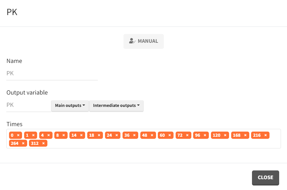
Parameter element

Population parameters (fixed & random effects) and the random-effect correlations are kept as in Li et al. The only additions for Part 2 are: formulation-effect coefficients beta_Fsc_FORM_T​, beta_Cl_FORM_T, beta_Kd_FORM_T (initialized to 0 in the template and updated in R to implement test-product perturbations), and IOV standard deviations gamma_ksc, gamma_Fsc and gamma_kp for the occasion-level random effects (set to 0.2, i.e., 20% period-to-period variability).

R automation and simulation scenario generation

In this section, we describe the elements that change from simulation scenario to simulation scenario and are automatically updated by an R script.

Parameter perturbations

Product-difference scenarios are defined as percent changes applied to one parameter at a time:

• Fsc​: 0, 2, 4, 6, 8, 10%

• CL, Kd​: 0, 5, 10, 25, 50, 75, 100, 125, 150%

For each scenario, the automation script selects (i) which coefficient to change (beta_Fsc_FORM_T, beta_Cl_FORM_T, or beta_kd_FORM_T) and (ii) the corresponding percent change (fold). The script then updates the chosen beta value accordingly, while keeping all other beta values at 0.

Importantly, these beta coefficients are linked to the formulation covariate FORM:
the updated beta only modifies the parameter when FORM='T' (test). For FORM='R' (reference), the formulation effect is zero, so the reference parameter value is unchanged.

# beta fold calculation (one parameter at a time)
if (param %in% c("beta_kd_FORM_T", "beta_Cl_FORM_T")) {
  # Kd and CL are lognormal: multiplicative change on natural scale
  popParam_mod <- popParam_base %>% 
    mutate(!!param := .data[[param]] + log(1 + fold/100))
  # Fsc is logit-normal on (0,1): apply multiplicative change on Fsc_pop and convert to logit shift

} else if (param == "beta_Fsc_FORM_T") {
  popParam_mod <- popParam_base %>%
    mutate(!!param := .data[[param]] +
             (log(((1 + fold/100) * Fsc_pop) / (1 - (1 + fold/100) * Fsc_pop)) -
              log(Fsc_pop / (1 - Fsc_pop))))
}

Occasion element (two occasions per subject)

The two-period crossover structure is implemented by defining an occasion table with two occasions (occ = 1, 2) for every subject.

# create occasion element
  df_occ <- data.frame(occ    = rep(occ, each = nb_sbj), # nb_sbj = number of subjects
                       id     = 1:nb_sbj,
                       time   = 0)
  file_name <- tempfile("occs", fileext = ".csv")
  write.csv(df_occ, file_name, row.names = FALSE)
  defineOccasionElement(element = file_name)

Covariate elements and simulation groups

Because FORM is included in the model as a formulation covariate effect, the automation workflow can generate covariate tables that assign FORM per subject and per occasion to implement the RT/TR crossover sequences. In the same tables, WT is generated once per subject and repeated across both occasions so it remains constant within-subject. A lognormal distribution is assumed, with a typical weight of 70 kg and a standard deviation of 20%. The resulting long-format datasets (id, occ, FORM, WT) are written to CSV and registered in Simulx as covariate elements for the two sequence groups.

# Define Treatment sequence for simulation groups
FORM_seq_RT <- data.frame(occ  = rep(occ, each = nb_sbj),
                          id   = 1:nb_sbj,
                          FORM = rep(c("R", "T"), each = nb_sbj))# 1st occ = R, 2nd occ = T
FORM_seq_TR <- data.frame(occ  = rep(occ, each = nb_sbj),
                          id   = 1:nb_sbj,
                          FORM = rep(c("T", "R"), each = nb_sbj))# 1st occ = T, 2nd occ = R
# Define Weight
WT_RT_val <- round(rlnorm(nb_sbj, meanlog = log(70), sdlog = 0.2),0)
WT_RT <- data.frame(id = 1:nb_sbj, WT = WT_RT_val)
    
WT_TR_val <- round(rlnorm(nb_sbj, meanlog = log(70), sdlog = 0.2),0)
WT_TR <- data.frame(id = 1:nb_sbj, WT = WT_TR_val)
    
# Combine RT-WT and TR-WT
RT <- merge(FORM_seq_RT, WT_RT, by = "id")
TR <- merge(FORM_seq_TR, WT_TR, by = "id")
    
# create covariate elements RT & TR (with WT)
file_name <- tempfile("RT", fileext = ".csv")
write.csv(RT, file_name, row.names = FALSE)
defineCovariateElement(name = "RT", element = file_name)
    
file_name <- tempfile("TR", fileext = ".csv")
write.csv(TR, file_name, row.names = FALSE)
defineCovariateElement(name = "TR", element = file_name)

Replicates

Replicates are used to estimate power as the fraction of trials that would pass BE. Within a scenario, most elements are held fixed (model, treatment, two-occasion structure, and the scenario-specific parameter perturbation), and only the random seed changes between replicates. Replicates are simulated immediately at the largest sample-size batch, i.e., on all subjects (e.g., 125 subjects per sequence group) to generate one complete trial dataset per replicate.

After all replicates are simulated, sample-size evaluation is performed with a nested loop: the outer loop iterates over the sample-size batches (j in 25, 50, 75, 100 and 125), and the inner loop iterates over replicates. For each batch size j, the script selects j unique subject IDs from the replicates using sample(all_ids, j) (default without replacement), and runs the PKanalix NCA/BE workflow.

set.seed(123)  # for subject group sampling
  all_ids <- sort(unique(rep_all$original_id))
  for (j in vec_sbj) {
    for (rep_2 in 1:nb_reps) {
      sampled_ids <- sample(all_ids, j) # random selection of j subjects
      data_j <- rep_all %>% filter(original_id %in% sampled_ids, rep == rep_2)
      
      write.csv(data_j, paste0(path.prog, "/2_tempProject/Simulation/simulatedData_perIdRep.csv"), row.names = FALSE)
      datafile <- file.path(paste0(path.prog, "/2_tempProject/Simulation/simulatedData_perIdRep.csv"))

      initializeLixoftConnectors(software = "pkanalix")
      message(sprintf(
        "[INFO] Starting iteration: param=%s | fold=%s | nb=%d | rep=%d", param, fold, j, rep_2))
      
      newProject(data = list(dataFile = datafile,
                             headerTypes =c("id","occ","ignore", "time", "observation", "obsid", "amount", "contcov", "catcov", "catcov","ignore")))
      #------------------------------------------------------------------------------
      # NCA & BE setup: PK data
      setNCASettings(administrationType    = list("1"="extravascular"), 
                     integralMethod        = "upDownTrapUpDownInterp", # "linear up log down"
                     computedNCAParameters = c("AUCINF_obs","Cmax"),
                     startTimeNotBefore = list(TRUE, 100))
      setBioequivalenceSettings(computedBioequivalenceParameters = data.frame(parameters = c("AUCINF_obs", "Cmax"), logtransform = c(TRUE)),
                                linearModelFactors               = list(id          = "ID", 
                                                                        period      = "occ", 
                                                                        formulation = "FORM",
                                                                        reference   = "R",
                                                                        sequence    = "group"))
      setScenario(nca=TRUE, be=TRUE)
      setNCASettings(obsidtouse = "PK") # Conduct NCA& BE for PK data
      runScenario()
      # Retrieve results
      be_resultPK <- getBioequivalenceResults()$confidenceIntervals$`T` %>%
        mutate(param   = param,
               fold    = paste0(fold,"%"),
               nb_subj = j,
               rep     = rep_2,
               metric  = "PK") %>%
        select(-AdjustedMean_T, AdjustedMean_R, Difference, CIRawLower, CIRawUpper)
      #------------------------------------------------------------------------------
      # Analoguously for PD data
      # ...
      #------------------------------------------------------------------------------
      results_all <- rbind(results_all, be_resultPK, be_resultPD)
    }
  }
write.csv(results_all, paste0(path.prog,"/Results/results_IOV20.csv"), row.names = FALSE)

This is repeated batch-by-batch from the smallest to the largest sample-size value.

Results

Delivered dose (Fsc) pertubations

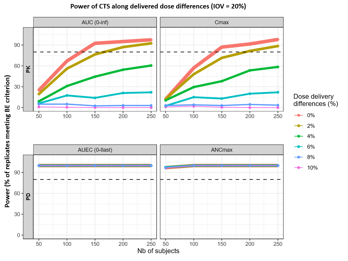
Delivered-dose differences primarily impact PK power, while PD endpoints (AUEC, ANCmax) consistently exceed 80% power across all scenarios. For PK metrics, reaching the 80% threshold is highly sensitive to dose magnitude: at 0% difference, the target is met with 125 subjects for AUC(0–inf) and 138 for Cmax. A 2% difference pushes these requirements to 167 and 192 subjects, respectively, with Cmax being the limiting endpoint. Beyond a 2% difference, PK power fails to reach 80% within the 50–250 subject range, staying below the threshold at 4% and remaining near zero at differences of 6% or higher.

Potency (Kd) pertubations

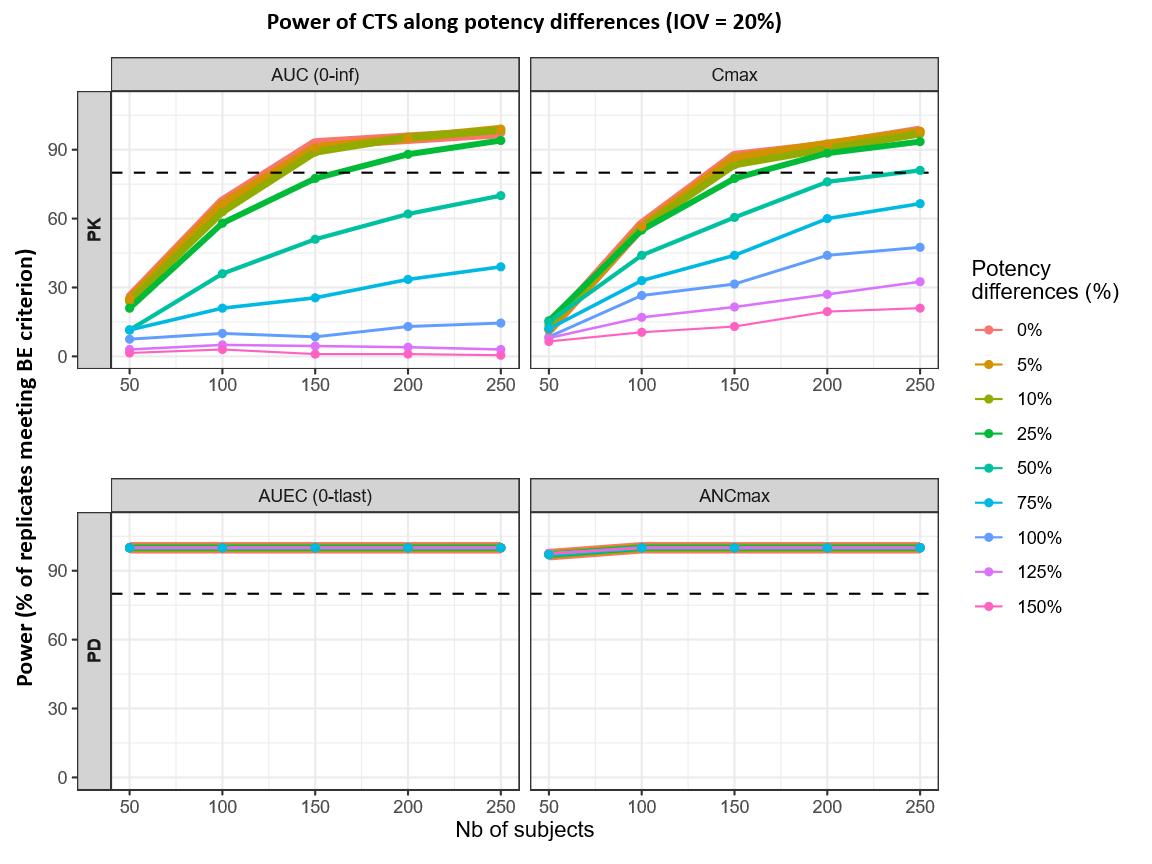
Potency differences primarily affect PK-based power, while PD endpoints (AUEC, ANCmax) remain close to 100% power across the full sample-size grid. In the PK panels, small potency differences are compatible with high power at moderate sample sizes: for 0–10% Kd differences, the 80% power threshold is reached at roughly 125–133 subjects for AUC(0–inf) and 138–144 subjects for Cmax. At a 25% Kd difference, the required sample size increases to about ~162 subjects for AUC(0–inf) and ~161 subjects for Cmax, with Cmax remaining the limiting endpoint overall as potency differences increase beyond this range.

Clearance (CL) pertubations

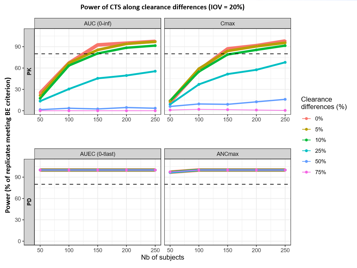
For clearance differences up to 10%, the sample size required to reach 80% power increases from 125 to 149 subjects for AUC(0–inf) and from 138 to 158 subjects for Cmax. Beyond this 10% threshold, power for the PK parameters drops so significantly that the 80% mark is never reached, even with a maximum sample size of 250 subjects. In contrast, the PD endpoints (AUEC and ANCmax) maintain near 100% power across all tested clearance differences and subject counts.

Conclusion

Across the simulated 6 mg, 2x2x2 crossover scenarios, PK endpoints determine the sample size needed to achieve the 80% power target for concluding BE. In contrast, PD endpoints meet the BE criterion across all explored scenarios and are therefore not discriminating in this analysis. This mirrors Part 1, where ANC-based metrics remained essentially unchanged under delivered-dose, potency (Kd), and clearance (Cl) perturbations, due to the coupled PK/PD feedback in pegfilgrastim, where ANC dynamics and receptor-mediated processes dampen PD variability even when exposure shifts are detectable.

Among the investigated product-difference drivers, delivered-dose differences (Fsc) are the most sample-size limiting: maintaining ~80% power at ≤2% delivered-dose difference requires approximately 200 subjects in total. For potency differences (Kd), ~150 subjects are sufficient to reach ~80% power for differences up to ~25%, and for linear clearance differences (Cl), ≥150 subjects are sufficient for differences up to ~10%.

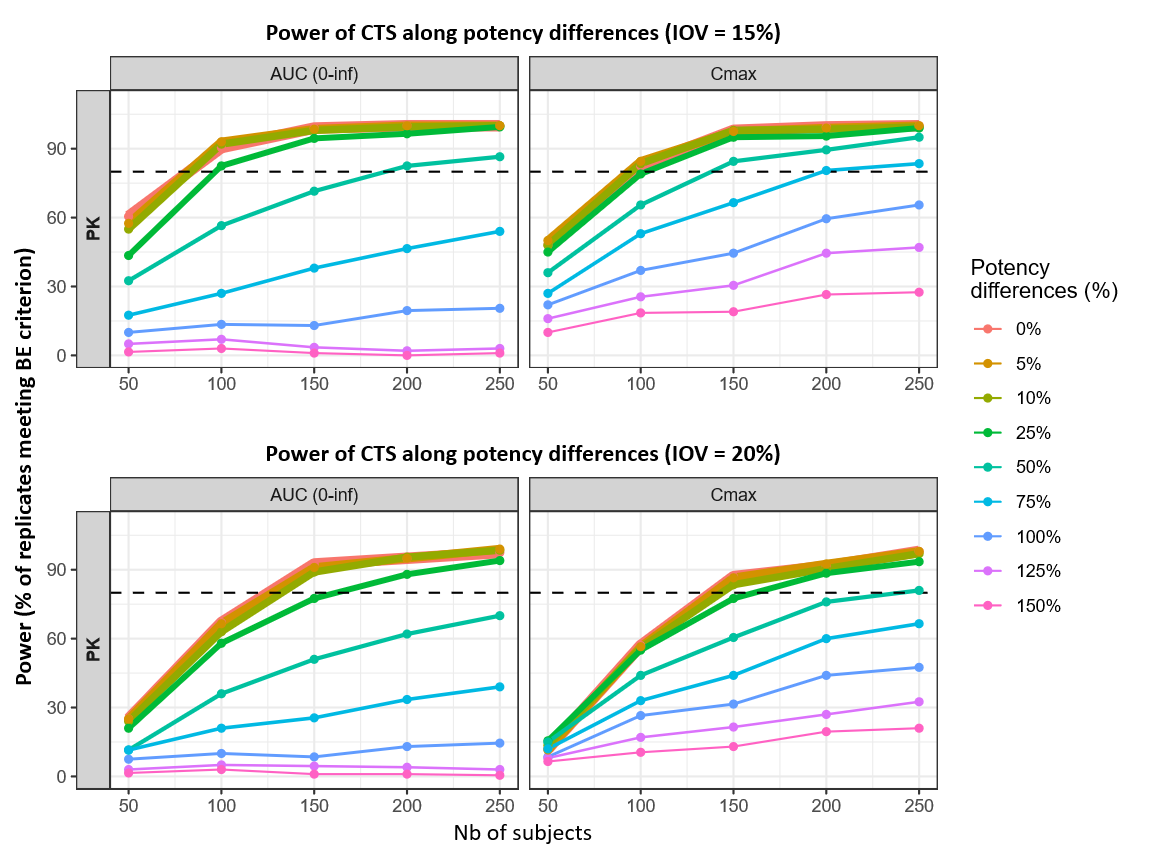
Impact of inter-occasion variability on power and sample size

Inter-occasion variability (IOV) represents within-subject, period-to-period changes in parameters such as absorption and delivered fraction in a crossover study. In these simulations, IOV is a main driver of the within-subject variability in the BE model; lowering IOV therefore increases power and reduces the sample size needed to reach the 80% target.

To illustrate this, two IOV levels are compared. IOV = 20% is used as a “typical clinical” scenario (higher real-world uncertainty in absorption/distribution), whereas IOV = 15% reflects a more controlled study environment. Across delivered-dose, clearance, and potency scenarios, the lower IOV consistently shifts PK (AUC, Cmax) power upward and the 80% power sample-size threshold downward.

Delivered dose (Fsc) pertubations

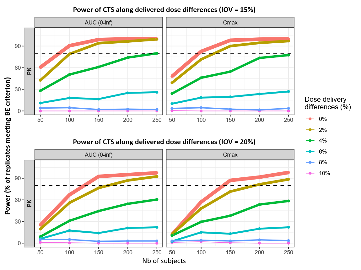
Reducing IOV from 20% to 15% shifts the PK power curves upward across delivered-dose scenarios, translating into smaller sample sizes to reach 80% power for AUC(0–inf) and Cmax. At 0% difference, the 80% threshold decreases from 125 → 82 subjects for AUC(0–inf) and from 138 → 96 subjects for Cmax. At 2% difference, the required sample size decreases from 167 → 103 for AUC(0–inf) and from 192 → 123 for Cmax.

For larger delivered-dose differences, power remains constrained: at 4%, AUC(0–inf) reaches 80% only at the upper end of the explored range (~250 subjects) under IOV 15%.

Potency (Kd) pertubations

Under the more controlled 15% IOV assumption, 0–25% potency (Kd) differences reach 80% power with about 82–97 subjects for AUC(0–inf) and 93–103 subjects for Cmax, compared with 125–162 (AUC) and 138–161 (Cmax) under 20% IOV.

The impact of IOV becomes even more pronounced for larger potency differences. At 50%, the 80% threshold decreases from ~240 subjects (Cmax, 20% IOV) to ~138 subjects (Cmax, 15% IOV); AUC(0–inf) shows a similar downward shift (~189 subjects at 15% IOV vs 20% IOV).

Clearance (CL) pertubations

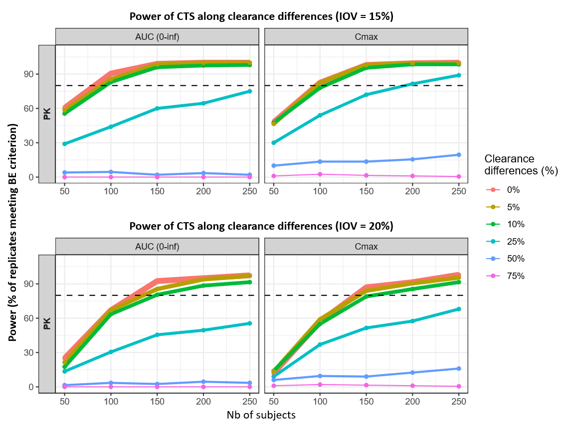
For linear clearance (CL) perturbations, lowering IOV from 20% to 15% reduces the sample size needed to reach 80% power across the clinically relevant 0–10% range. The 80% thresholds shift from 125 → 82 subjects for AUC(0–inf) at 0% difference and from 149 → 95 subjects at 10% difference; for Cmax, the corresponding shifts are 138 → 96 (0%) and 158 → 106 (10%).

Across these scenarios, Cmax remains the more sample-size limiting PK endpoint. At larger clearance differences, the curves illustrate a feasibility boundary within the explored grid: for example, at 25%, Cmax reaches 80% only at the upper end under 15% IOV (≈192 subjects), while higher differences remain well below the 80% target even with 250 subjects.

The robustness check shows that the assumed IOV level has a large impact on the predicted power and the sample size needed to reach 80% power. Using 15% instead of 20% IOV consistently leads to higher PK power and smaller required sample sizes for the same delivered-dose (Fsc), potency (Kd), or clearance (CL) scenario.

Therefore, reliable sample size recommendations depend on having a realistic IOV estimate (or at least a realistic range).

IOV should be taken from:

• published PopPK analyses under comparable conditions (dose, route, population, design, etc),

• a small pilot crossover study if suitable data are unavailable, and/or

• robustness checks over a plausible range (e.g., 10–25%). Overestimating IOV can inflate sample size; underestimating IOV risks an underpowered study.

Practical application: translating analytical similarity into trial power

This chapter provides a worked example of translating known, literature based test–reference differences into predicted trial power and sample size using the simulation workflow introduced in Part 2. Two complementary publications are used as inputs: an analytical similarity assessment reporting protein content (used to motivate an Fsc-type delivered-dose difference) and receptor-binding kinetics/affinity (used to define a Kd perturbation) (Brokx et al., 2017), and a confirmatory single-dose 6 mg, two-way crossover PK/PD similarity study in healthy volunteers used to benchmark the simulated sample size and to inform a comparative CL difference derived from the reported PK summary statistics (Desai et al., 2016).

The practical example applies Fsc, Kd, and CL differences, using the following literature-derived inputs (biosimilar minus reference): Fsc −1.0%, Kd −16.7%, and CL −1.8%.

• Fsc (delivered-dose factor) was motivated by the reported protein concentration difference measured by UV absorbance at 280nm (OD280): 9.9 ± 0.3 mg/mL (biosimilar) vs 10.0 ± 0.4 mg/mL (reference), corresponding to −1.0%.

• Kd (receptor-binding affinity) was taken from surface plasmon resonance (SPR) receptor-binding kinetics, where Kon/Koff and KD were estimated; the reported KD values were 150pM (biosimilar) vs 180pM (reference), giving −16.7%.

• CL (linear clearance) was taken from the confirmatory study’s PK NCA summary table, reported as geometric-mean–based PK parameters: 1185 mL/h (biosimilar) vs 1206 mL/h (reference), corresponding to −1.8%.

Fsc and Kd originate from the analytical similarity assessment (Brokx et al. 2017), whereas the CL difference is based on NCA-derived PK summaries from the confirmatory study (Desai et al. 2016) and is treated as a preliminary clinical estimate.

Simulation setup

The simulation workflow is the same as in Part 2 (same clinical trial simulation and bioequivalence decision framework), with the following modifications:

• Simultaneous parameter perturbations
  The literature-derived product differences for Fsc, Kd, and CL are applied simultaneously within each simulated replicate to reflect a combined, plausible “real-world” difference rather than isolated effects.

• IOV fixed to 15%
  Inter-occasion variability is fixed at 15%, consistent with the more optimistic IOV scenario.

• PK endpoints
  For PK, AUC(0–tlast) is used (instead of AUC(0–inf)) together with Cmax, to match the PK outcome definitions used in the confirmatory study analysis.

• PD Bioequivalence confidence interval
  For PD, the bioequivalence assessment uses a 95% confidence interval, consistent with the confirmatory study’s PD analysis.

Results

Multi-parameter perturbations (Fsc, Kd, CL)

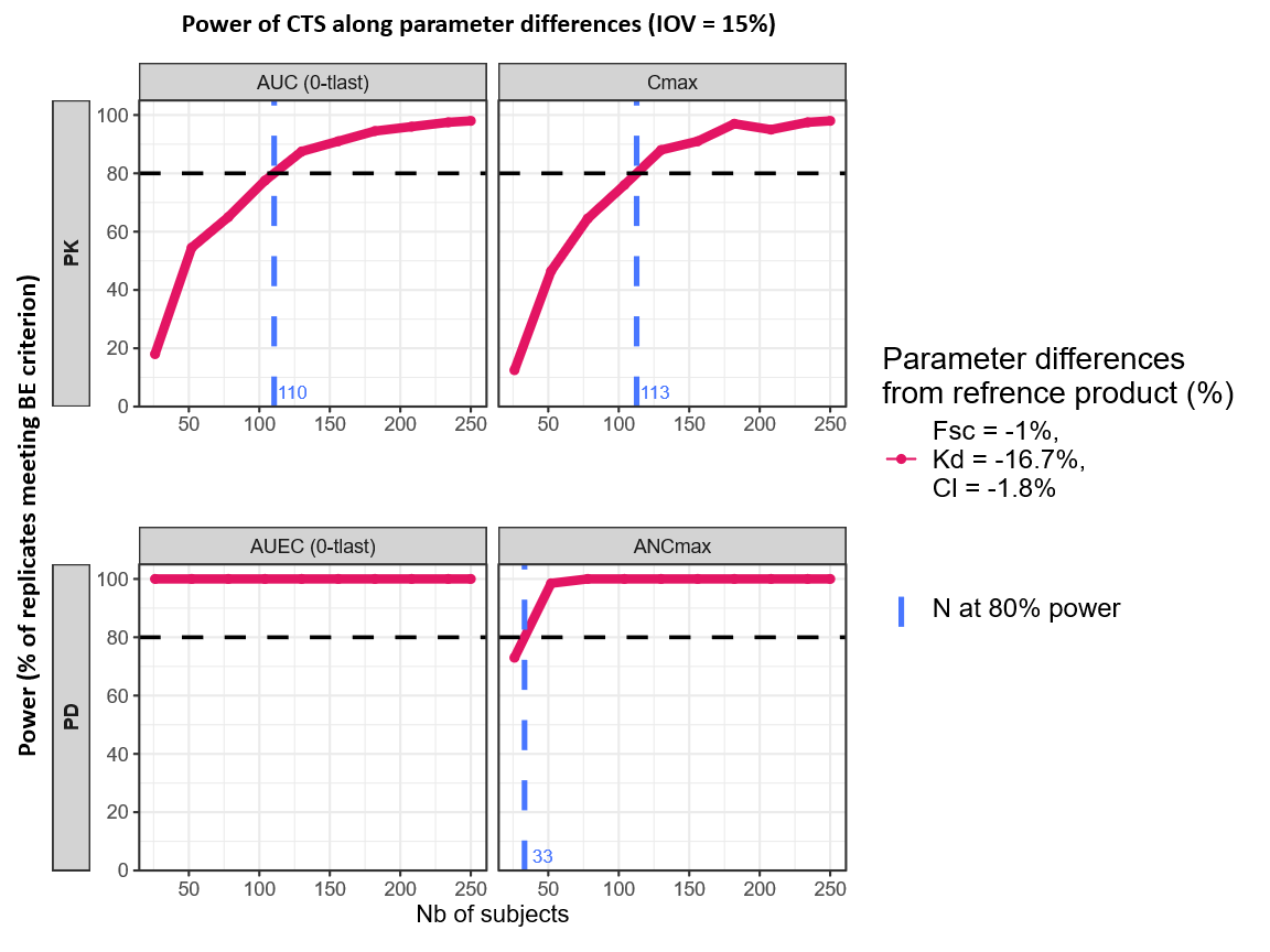
Across the four power curves (PK: AUC(0–tlast) and Cmax; PD: AUEC(0-tlast) and ANCmax), the combined literature-based scenario shows a consistent pattern: power increases with sample size. All endpoints exceed the 80% target within the explored range. The overall sample size required is led by the most limiting endpoint, which is Cmax, crossing 80% at interpolated ~113 subjects. The other endpoints reach 80% at smaller sample sizes (AUC(0–tlast) slightly below Cmax; PD endpoints substantially lower), so a total sample size of ~113 subjects provides ≥80% power.

In the confirmatory study (Desai et al., 2017), 112 subjects have been included (i.e., 56 subjects per sequence, RT and TR). Bioequivalence was concluded for the primary PK endpoints using 90% confidence intervals, and for the primary PD endpoints using 95% confidence intervals, both within 80–125% margins.

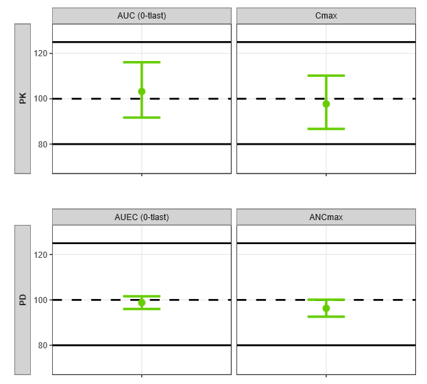
N = 112 Subejcts
Endpoints		Relative mean ratio	CI (PK: 90%, PD: 95%)
PK	AUC (0-tlast) (pg·h/mL)	103.2	91.7–116.1
	Cmax (pg/mL)	97.7	86.7–110.2
PD	AUEC (0-tlast) (cells x 109·h/L)	98.8	96.0–101.6
	ANCmax (cells x 109 /L)	96.3	92.6–100.1

All PK and PD endpoints satisfied the 80–125% criterion, and the plotted intervals are narrow relative to the acceptance limits, indicating clear separation from the margins under the chosen CI levels.

Using CAA-derived Fsc/Kd differences (with the CL difference from assumed preliminary data) as simultaneous inputs to the simulation workflow yielded an 80%-power sample size of ~113 subjects, closely matching the 112-subject confirmatory PK/PD similarity study outcome.

This practical example illustrates how the workflow can be applied to derive a sample size for a PK/PD biosimilarity study by translating known, literature-reported test–reference differences from into predicted power under the planned design and decision criteria.

Discussion

This case study is intended as a reusable template rather than a pegfilgrastim-only solution. The same workflow (mechanistic model selection, sensitivity analysis to identify design drivers, and clinical trial simulation to map variability and expected product differences to power) can be adapted to other biosimilars by updating the structural/statistical model, endpoints, and study design assumptions. For instance, the simulation can be reformulated for a parallel design when crossover is not appropriate, or extended to alternative dosing regimens and sampling schedules. In addition, the “product-difference scenarios” can be parameterized using e.g. evidence from a comparative analytical assessment (CAA) (e.g., translating analytically supported differences into model perturbations), enabling a quantitative link between expected differences and the sample size required for an adequately powered comparative PK/PD similarity study.