Tobramycin dose individualization

In this example modeling and simulation workflow, we model tobramycin pharmacokinetics and simulate dosing regimens in patients with various degrees of renal function impairment.

Introduction

Overview

Tobramycin is an antimicrobial agent of the aminoglycosides family, which is among others used against severe gram-negative infections. Because tobramycin does not pass the gastro-intestinal tract, it is usually administrated intravenously as intermittent bolus doses or short infusions.

Tobramycin is a drug with a narrow therapeutic index. For efficacy, a sufficiently high serum concentration must be achieved. On the other hand, an excess exposure over a long time period bears the risk of nephrotoxicity and ototoxicity.

By developing a population pharmacokinetic model for tobramycin, and relating the pharmacokinetic parameters to easily accessible covariates such as creatinine clearance (representative of the kidney filtration rate) and body weight, the inter-individual variability can be better understood. It is then possible to use this information to a priori determine the best dosing regimen for an effective and safe concentration, using the patient covariate values. This constitutes an example of personalized medicine.

In addition, a rapid assay is available to measure serum tobramycin concentrations. Hence, by monitoring the drug concentration at a few time points after the first dose, the individual PK parameters can be estimated and used to adapt the subsequent doses. The optimal times for the drug monitoring can also be assessed, as an example of optimal design.

The data set presented in this case study has been originally published in:

Aarons, L., Vozeh, S., Wenk, M., Weiss, P. H., & Follath, F. (1989). Population pharmacokinetics of tobramycin. British journal of clinical pharmacology, 28(3), 305-314.

and a case study is presented in:

Bonate, P. L. (2006). Nonlinear Mixed Effects Models: Case Studies. Pharmacokinetic-pharmacodynamic modeling and simulation (pp. 309-340). New York: Springer.

Workflow

We will first explore the data set with Monolix to better grasp its properties. We will then go through the model building process and implement the model in the Mlxtran language in Monolix, estimate the parameters, and assess the model using the built-in diagnostic plots. Once a satisfactory model is obtained, simulations of new dosing regimens for specific patients or patient populations will be done using Simulx.

Exploratory data analysis with Monolix

Data set overview

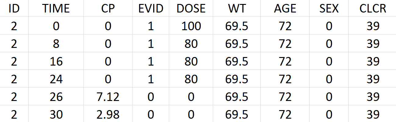
Tobramycin bolus doses ranging from 20 to 140mg were administrated every 8 hours in 97 patients (45 females, 52 male) for 1 to 21 days (for most patients, for ~6 days).  Age, weight (kg), sex, height and creatinine clearance (mL/min) are available as covariates. Because height information was missing for around 30% of the patients, this covariate is ignored. The tobramycin concentration (mg/L) was measured 1 to 9 times per patients (322 measures in total), generally between 2 and 6h post-dose. Below is an extract of the data set file:

• ID: identifier of the patients

• TIME: time of dose or measurement (hours)

• CP: Tobramycin plasma concentration (mg/L)

• EVID: event identifier, 0=measurement, 1=dose

• DOSE: amount of the dose (mg)

• WT: weight (kg)

• AGE: age (years)

• SEX: 1=male, 0=female

• CLCR: creatinine clearance (mL/min)

Data set visualization with Monolix

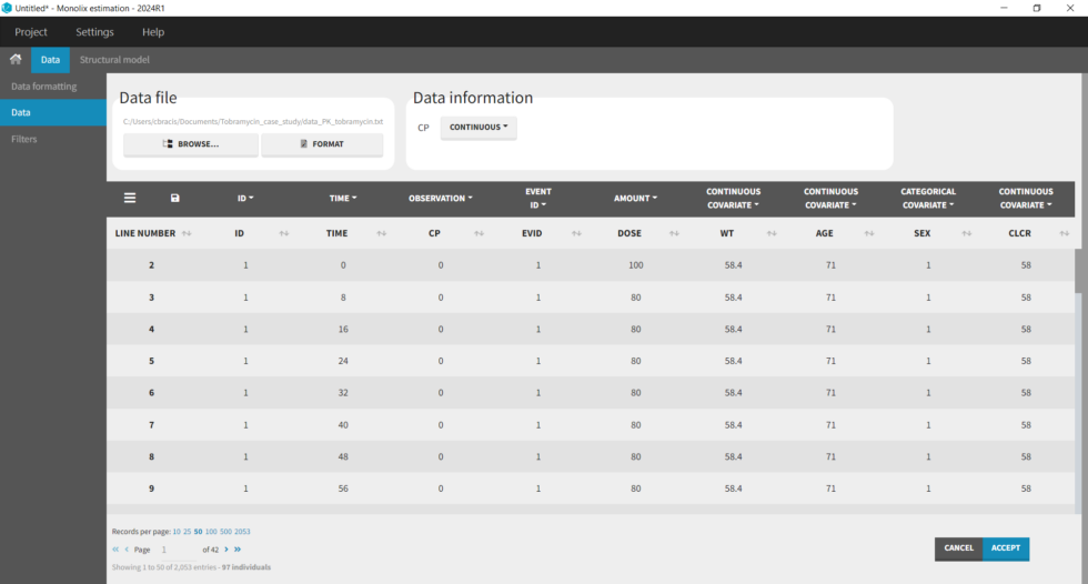
We first start exploring the data set in Monolix. After having opened Monolix, we create a new project and load the data set. Based on the header, most columns are automatically recognized. The column-type must be set manually for the observed concentration (CP column set to column-type OBSERVATION), the dose (DOSE column set to column-type AMOUNT), and the creatinine clearance (CLCR column set to column-type CONTINUOUS COVARIATE for continuous covariate):

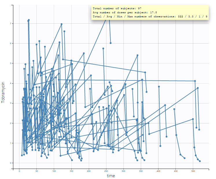
After accepting the data mapping and clicking on the Plots tab, the spaghetti plot is displayed (figure below). It is possible to split or filter the plot using the covariates, which in the present case does not show any meaningful insights.

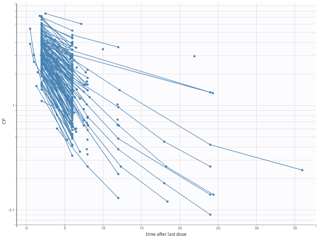
To have a closer look at the elimination kinetic, we can examine only the last dose by setting the “Time after last dose” option for the x-axis and plotting the y-axis in log-scale. We observe the following kinetics.

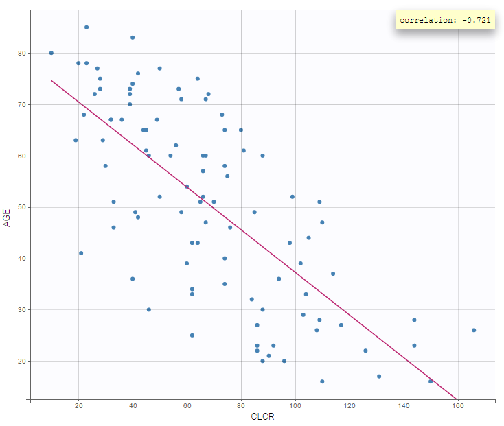
It is also interesting to display one covariate against another one. We, in particular, observe a negative correlation between age and creatinine clearance (correlation at -0.7):

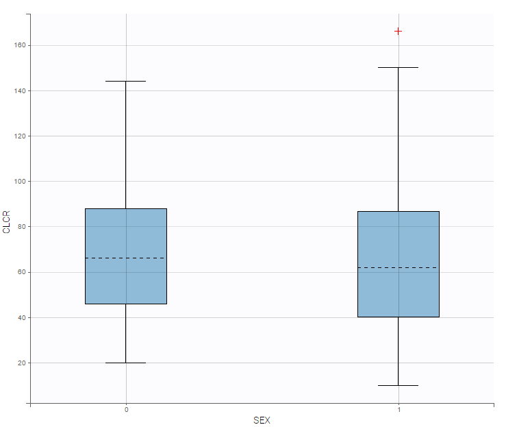
On the other hand, the creatinine clearance is similar for both sexes:

In summary, from the exploratory data analysis, we have gained the following insights:

• A 1 compartment model with linear elimination is a good first approximation, and we can also explore a 2 compartment model.

• Older patients have a lower creatinine clearance.

Model development with Monolix

Set up of a Monolix project: definition of data, structural and statistical model for the initial model

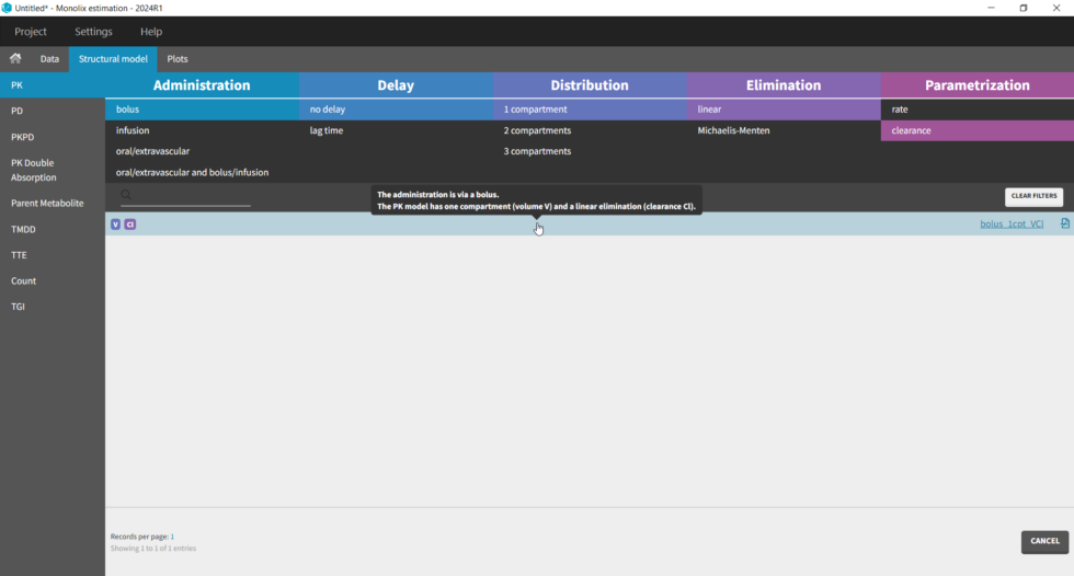
The setup of a Monolix project requires to define the data set, and the model, both the structural part and the statistical part, including the residual error model, the parameter distributions (variance-covariance matrix) and the covariate model. We will setup a first model and improve it step-wise. We first create a new project in Monolix and load the data, assigning the columns as we have done in Datxplore. After having clicked “Next”, the user is prompted to choose a structural model. As a first guess, we try a one-compartment model with bolus administration and linear elimination. This model is available in theMonolix PK library, which is accessed when clicking on “Load from Library > PK”. A (V,Cl) and a (V,k) parameterization are available. We choose the V,k one:

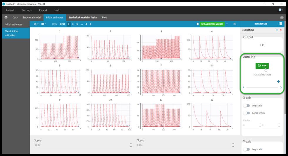
Selecting a model brings us to the next tab “Check initial estimates”, where the user can choose initial parameter values. Although Monolix is fairly robust with respect to initial parameter values, it is good practice to set reasonable initial values as this will speed up the convergence. The simulations with the population parameters are shown as red lines with blue points for the data for each individual. One can play with the values of V and Cl. However, because the data are sparse, it is not easy to find good initial values, though we see that increasing the values for V and Cl improves the fit. We can also try Monolix’s automated search for initial values, Auto-init. Under Auto-init in the right panel, first click the red x to remove the selected IDs (this will run auto-init on all individuals), then click the green Run button. The previous values (which can be recovered by clicking “#1 (INITIAL)” under References) are shown with dotted lines and the new auto-init estimates with solid lines. Don’t forget to click Set As Initial Values at the top of the window to save the current values as the initial estimates.

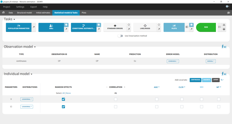
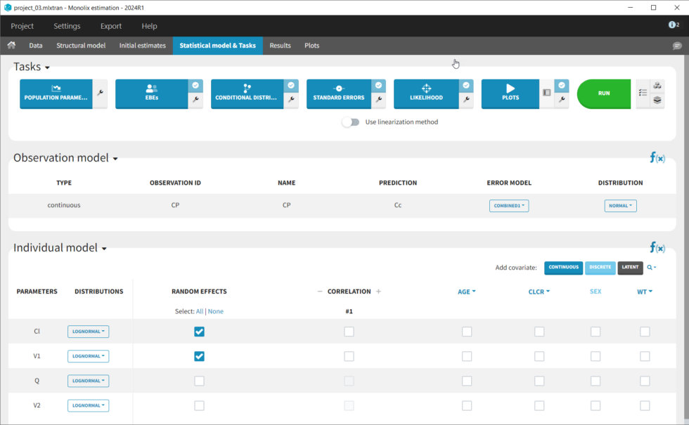
This brings us to the Statistical model & Tasks tab where we can setup the statistical part of the model and run estimation tasks. Under “Observation model,” we define the residual error model. We start with the default combined1 model with an additive and a proportional term, and we will evaluate alternatives later. Under “Individual model,” we define the parameter distributions. We keep the default: log-normal distributions for V and Cl, and no correlations. For now we ignore the covariates.

Now that we have specified the data and the model, we save the project as “project_01” (menu: Project > Save). The results files of all tasks run will be saved in a folder next to the project file. All Monolix project files can be downloaded at the end of this webpage.

Running tasks

A single task can be run by clicking on the corresponding button under Tasks. To run several tasks in a row, tick the checkbox in the upper right corner of each task you want to run (it will change from white to blue) and click the green run button. After each task, the estimated values are displayed in the Results tab and output as text files in the result folder with the same name as and next to the Monolix project.  

Estimation of the population parameters

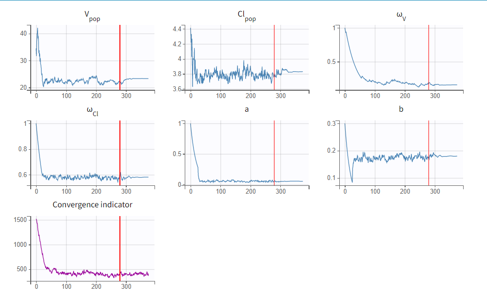
To run the maximum likelihood estimation of the population parameters, click on the Population Parameters button under Tasks. In the pop-up window, you can follow the progress of the parameter estimates over the iterations of the stochastic approximation expectation-maximization (SAEM) algorithm. This algorithm has been shown to be extremely efficient for a wide variety of even complex models. In a first phase (before the red line), the algorithm converges to the neighborhood of the solution, while in the second phase (after the red line) it converges to the local minimum. By default, automatic termination criteria are used. In the current case, the algorithm shows good convergence:

The estimated population parameter values can be accessed by clicking on the Results tab and are also available in the results folder as populationParameters.txt.  

Estimation of the EBEs

The EBEs (empirical Bayes estimates) represent the most probable value of the individual parameters (i.e., the estimated parameter value for each individual). These values are used to calculate the individual predictions that can be compared to the individual data to detect possible mis-specifications of the structural model, for instance. After running this task, the estimated parameter values for each individual is shown in the Results tab and are also available in the results folder > IndividualParameters > estimatedIndividualParameters.txt.  

Estimation of the conditional distribution

The individual parameters are characterized by a probability distribution that represent the uncertainty of the individual parameter values. This distribution is called the conditional distribution and is specified

. The EBEs are the most probable value of this probability distribution. When an individual has only few data points, the probability distribution may be very large (i.e., large uncertainty). In this case, the EBE values tend to be similar to the population parameter values (shrinkage phenomenon, learn more here) and does not properly represent the individual. The task “Conditional Distribution” samples several (by default 10) possible individual parameter values from the conditional distribution using an MCMC procedure. These values provide a more unbiased representation of the individuals and improve the diagnostic power of the plots.  

Estimation of the standard errors, via the Fisher Information Matrix

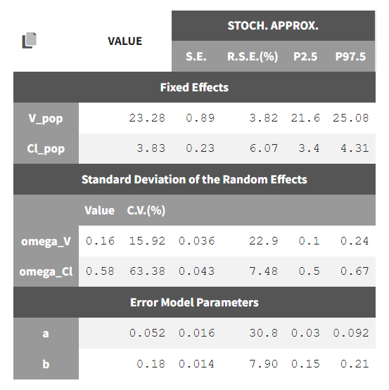
To calculate standard errors of the population parameter estimates, one can calculate the Fisher Information Matrix (FIM). Two options are proposed: via linearization (toggle “Use linearization method” on) or via stochastic approximation (toggle off). The linearization method is faster but the stochastic approximation is usually more precise. As our model runs quickly, we can afford to select the stochastic approximation option and click on the Standard Errors button to calculate the FIM. After the calculation, the standard errors are added to the population parameter table:

Estimation of the log-likelihood

For the comparison of this model to more complex models later on, we can estimate the log-likelihood, either via linearization (faster, toggle “use linearization method” on) or via importance sampling (more precise, toggle off). Clicking on the Likelihood button under Tasks (with “use linearization method” unchecked), we obtain a -2*log-likelihood of 668, shown in the Results tab under Likelihood, together with the AIC and BIC values. By default, the Standard Errors and Likelihood tasks are not enabled to run automatically. We can click the checkbox to the right of each button to run them automatically when we click the Run button in the future.  

Generation of the diagnostic plots

To assess the quality of the model, we finally can generate standard plots. Clicking on the icon next to the Plots button under Tasks, one can see the list of possible figures. Clicking on the Plots button generates the figures.  

Model assessment using the diagnostic plots

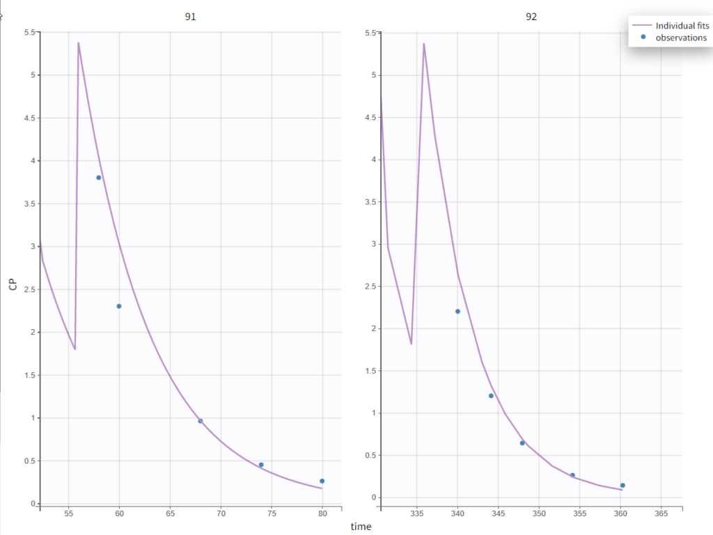
In the “Individual fits” plot, you can choose which individual(s) and how many you would like to display using the buttons in the upper left above the plots:

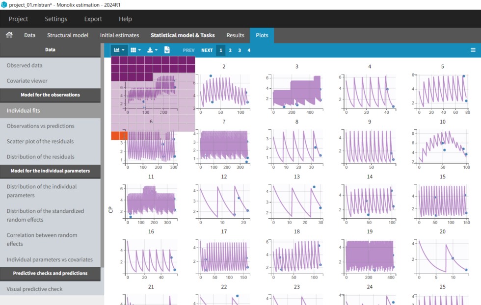
It’s possible to zoom in on a zone of interest, which is particularly useful for such sparse data sets. This can be done by 1) under Axes on the right panel, setting custom limits for the x-axis or 2) dragging a rectangle where you would like to zoom in on the plot itself (a double-click will zoom back). Here, for instance, are the last time points for individuals 91 and 92:

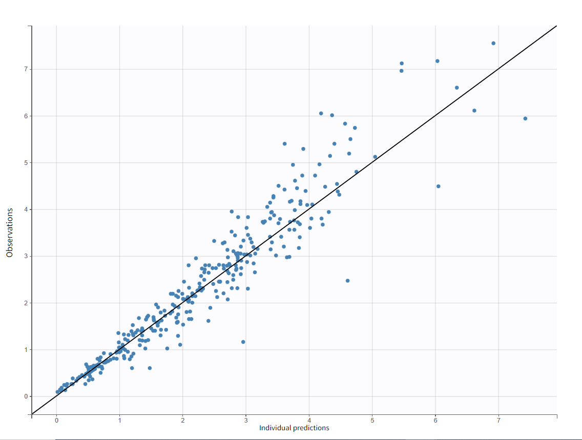
The “Observations vs Predictions” plot also looks good:

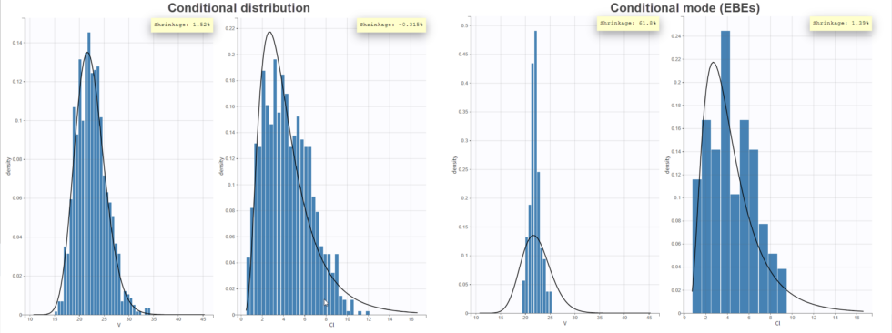
In the “Distribution of the individual parameters”plot, the theoretical parameter distributions (using the estimated population parameters, shown with the line) can be compared to the empirical distribution of individual parameters (histogram). In the Settings section of the right panel, under display, you can choose how to display the individual parameters in the histogram. With the “conditional distribution” option (the default), the individual parameters are drawn from the conditional probability to obtain an unbiased estimator of . This allows better detection of parameter distribution mis-specifications. With the “conditional mean” or “conditional mode (EBEs)” options, the shrinkage (specifically the -shrinkage, based on the among-individual variation in the model) can be seen (click on “Information” in the General section to display it). The large shrinkage for V means that the data does not allow us to correctly estimate the individual volumes (right side of plot below). Note that the shrinkage is calculated differently in Nonmem and Monolix, see here for more details.

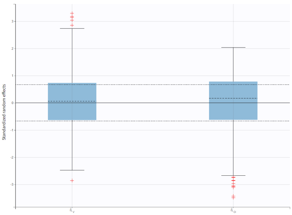
In the “Distribution of the standardized random effects”plot, the standardized random effects plotted as a boxplot are in agreement with the expected standard normal distribution (horizontal lines represent the median and quartiles). So there is no reason to reject the model due to the random effects:

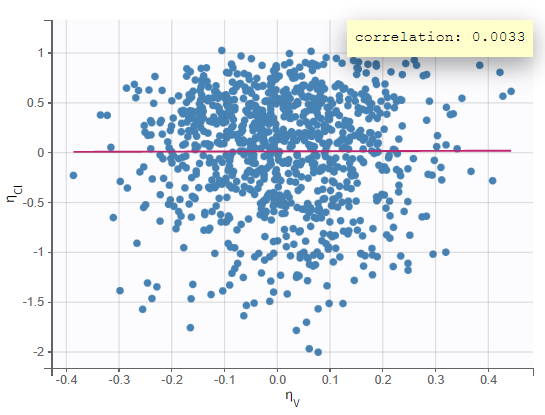
In the “Correlation between random effects”plot, the random effects of the two parameters are plotted against each other. No clear correlation can be seen.

We will look at the “Individual parameters vs covariates” plot later when we examine including covariates in the model. The “Visual predictive check” plot allows comparing empirical and theoretical quantiles to check for model misspecification. Given the variability in individual dosing times, we can turn on the option “Time after last dose” and put the y-axis on a log scale in the Axes settings in the right panel. Areas of mismatch are shown in red, and we can see some issues with predicting the peak and the final decline. Perhaps a two-compartment model would be a better structure for this data.  

Test of a two-compartment model

We thus change the structural model to the bolus_2cpt_ClV1QV2 model from the library. We save as project_02 and run the model. Quickly looking at the diagnostic plots, we don’t see any major changes and see that we still have issues fitting the peak in the visual predictive check. However, the -2*LL has dropped to 642. As our data is sparse, we will also try removing the variability on Q and V2, by unselecting the random effects. In this case, all subjects will have the same parameter value for Q and V2 (no inter-individual variability). We save as project_03 and run the model.

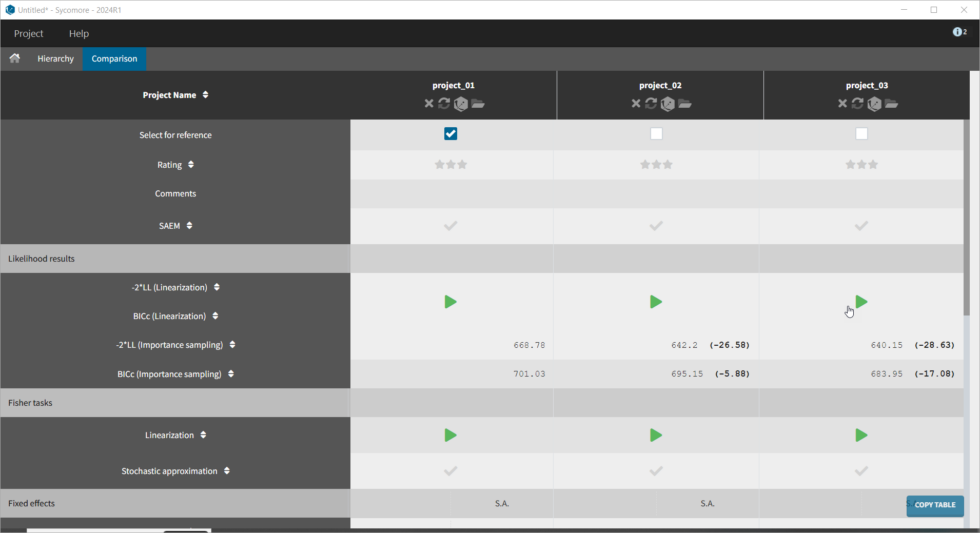
We can use Sycomore to compare the different versions of the model we’ve created thus far. To do so, create a new project and select the folder containing the mlxtran project files. One we select the projects in the tree at left, there is a table easily allowing us to see metrics for the selected projects.

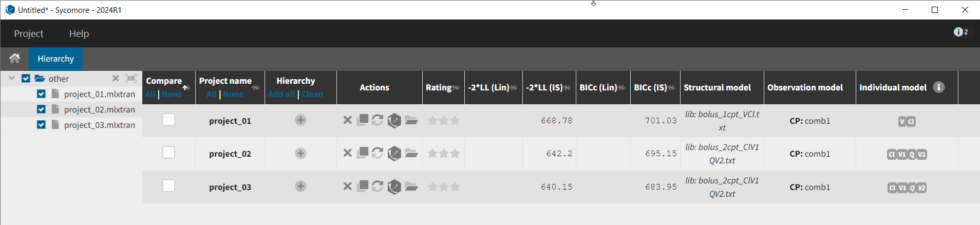
Furthermore, if we select the three models by clicking in the Compare column, then click on the Comparison tab, we get a table comparing likelihood and parameter values across models. We can select the first model as the reference, and note that the two compartment model without variability for Q and V2 (project_03) is significantly better (Δ-2*LL=29 and ΔBICc=17).

Adding covariates to the model

To get an idea of the potential influence of different covariates, we can look at the “Individual parameters vs covariates” plot, where the transformed parameters (log(V) and log(k) as we have chosen log-normal distributions) are plotted against the covariate values. Notice that we use the option “conditional distribution”. This means that instead of using the mode or mean from the post-hoc estimation of each individual parameter, we are sampling from its distribution. This is critical because it is known that the plots using the mode or mean of the post-hoc distribution often show non-existing correlations (see Lavielle, M. & Ribba, B. Pharm Res (2016)).

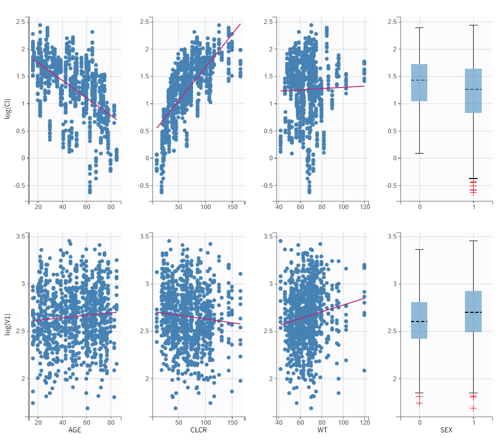
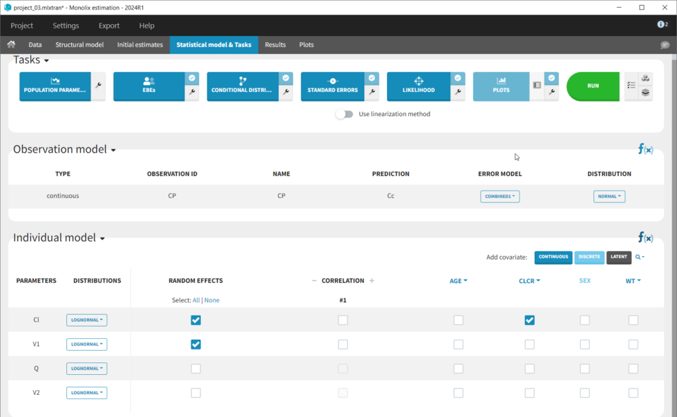
The covariates figure shows that log(Cl) decreases with AGE and increases with CLCR. It is possible to display the correlation coefficients in the Settings pop-up window, by selecting “Information”. Remember that during the exploratory data analysis, we noticed a negative correlation between AGE and CLCR. From a biological point of view, a correlation between Tobramycin clearance and creatinine clearance makes sense, as tobramycin is mainly cleared via the kidney. Thus we will try adding CLCR as covariate on the elimination parameter Cl. We will add covariates one by one, and thus consider other possible covariates afterwards. Before adding covariates, we click “Use the last estimates: All” in the Initial estimates tab, to re-use the last estimated parameter values as starting point for SAEM. To add the CLCR covariate on the parameter Cl, click on the corresponding checkbox under “Individual model” in the Statistical model & Tasks tab:

The corresponding equation can be seen by clicking on the formula button f(x) on the right: log(Cl) = log(Cl_pop) + beta_Cl_CLCR*CLCR + eta_Cl. So the covariate is added linearly to the transformed parameter. Rewritten, this corresponds to an exponential relationship between the clearance Cl and the covariate CLCR:

with sampled from a normal distribution of mean 0 and standard deviation . In the “Individual parameters vs covariates” plot, the increase of log(Cl) with CLCR is clearly not linear. So we would like to implement a power law relationship instead:

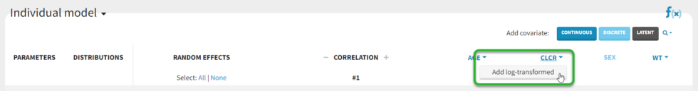
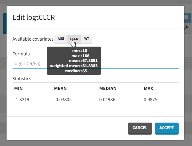
which in the log-transformed space would be written: log(Cl)=log(Cl_pop) + beta_Cl_CLCR*log(CLCR/65) + eta_Cl. Thus, instead of adding CLCR linearly in the equation, we need to add log(CRCL/65). We will create a new covariate logtCLCR = log(CLCR/65). Clicking on the triangle left of CLCR, then “Add log-transformed” creates a new covariate called logtCLCR.

Clicking the triangle right of the new logtCLCR covariate allows us to edit it. The weighted mean is used to center the covariate by default. However, this can be changed to another reference value by editing the formula. The centering ensures that Cl_pop is representative of an individual with a typical CLCR value (65 in our case). To help choose a centering value, hover over the covariate names to see the min, median, mean, and max over the individuals in the data set.

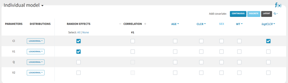
We then add logtCLCR as covariate to Cl, by clicking on the checkbox corresponding to logtCLCR in the row for parameter Cl.

In NONMEM, one would typically write:

TVCL = THETA(1)*((CLCR/65)**THETA(2))
CL = TVCL * EXP(ETA(1))

with THETA(1)=Cl_pop, THETA(2)=beta and std(ETA(1))= omega_Cl. In Monolix, we think in terms of transformed variables:

but the two models (in Nonmem and Monolix) are the same, corresponding to:

with sampled from a normal distribution of mean 0 and standard deviation . We now save the project as project_04, to avoid overwriting the results of the previous run. We then select all estimation tasks and click on Run to launch the sequence of tasks (Population Parameters, EBEs, Conditional Distribution, Standard Errors, Likelihood, and Plots). In the Results tab, loking at the population parameters, the effect on CLCR on k is fairly large: for an individual with CLCR=40 mL/min (moderate renal impairment) Cl = 2.6 L/hr, while for an individual with CLCR=100 mL/min (normal renal clearance) Cl = 5.7 L/hr. 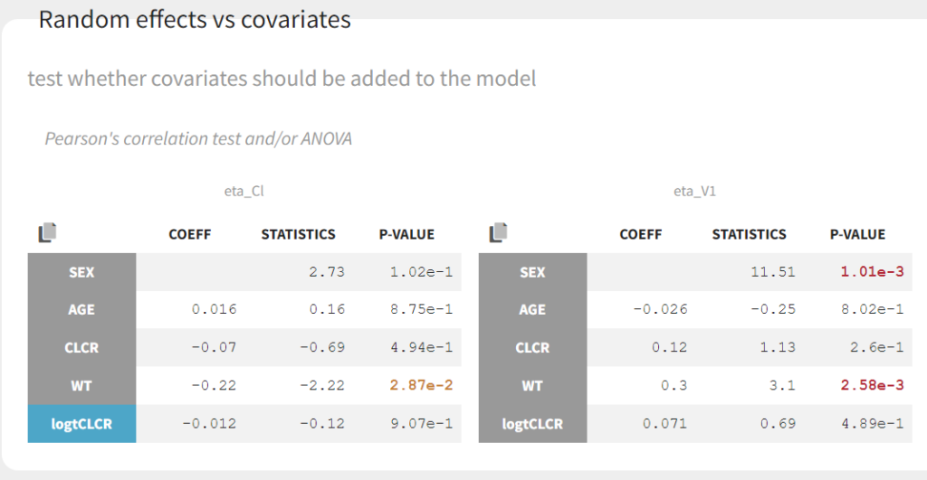In addition, the standard deviation of Cl omega_Cl has decreased from 0.56 to 0.31, as part of the inter-individual variability in Cl in now explained by the covariate. Clicking on Tests on the left shows the results of statistical tests to evaluate adding or removing covariates from the model. under “Individual parameter vs covariates,” we see the results of the correlation test and the Wald test to test whether covariates should be removed from the model. Both tests have a small p-value (< 2.2e-16) for the beta_k_logtCLCR parameter, meaning that we can reject the null hypothesis that this parameter is 0. Under “Random effects vs covariates,” there is a table of tests evaluating adding potential covariates to the model using Pearson’s correlation for continuous covariates and a one-way ANOVA for categorical covariates. Under eta_Cl, logtCLCR is shown in blue, showing it is already accounted for in the model and thus its p-value in non-significant. Small p-values are highlighted in red/orange/yellow and suggest testing the corresponding parameter-covariate relationship if it also makes biological sense. Note that the correlation tests are performed using the samples from the conditional distribution, which avoids bias due to shrinkage. To learn more about how Monolix circumvents shrinkage, see here. The results suggest are three potential covariate relationships to consider: WT on Cl, SEX on V1, and WT on V1. However, because sex and weight are likely correlated (which we can check in the “Covariate viewer” plot), and biologically it would make sense that weight would be correlated with volume, we will first try WT on V1.

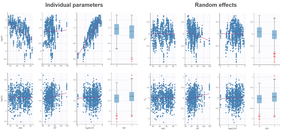
We can also look at the covariate relationships visually in the “Individual parameters vs covariates” plot. By plotting the random effects rather than the individual parameters, we can check for remaining correlations (option “Random effects” under “Display”). Note that no correlation is seen anymore between eta_Cl and AGE, as expected, as AGE and CLCR are strongly negatively correlated. In agreement with the statistical test, it appears that eta_Cl and eta_V1 are potentially correlated with the weight WT.

We could add either WT or logWT on log(V1). We choose to log-transform and center WT by 70, and add it as a covariate on log(V1). We save the project as project_05 and run the sequence of tasks again. The statistical tests show that beta_V1_logtWT appears to be significantly different from 0. Additionally, WT is no longer suggested as a covariate for eta_Cl though SEX is still proposed for eta_V1 even after taking weight into account. Note that the statistical tests and plots are giving indications about which model to choose, but the final decision lies with the modeler. We can also examine the projects with covariates in Sycomore to easily compare how the -2LL/BIC values and parameter estimates are changing with the covariates. We see that adding CLCR as a covariate to Cl significantly improved the model compared to the base 2 compartment model (Δ-2LL=105 and ΔBICc=101), and that additionally adding weight as a covariate to V1 was even better significantly better (Δ-2LL=120 and ΔBICc=111). The population parameter estimates for this model (project_05) are the following and -2LL is 520.

Automated covariate search

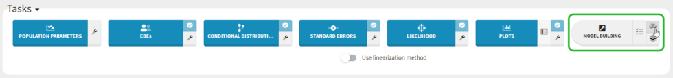
We could continue testing covariates one by one, by for example testing SEX as a covariate for V1. However, Monolix also provides several methods for automatically searching for covariates. These are accessed by clicking the button “Model Building” (three blocks) to the right of the Run button.

There are three different methods: SCM, which is a classic step-wise modeling approach, thorough but slow; COSSAC, which uses Pearson’s correlation and ANOVA tests to evaluate which covariates to test in forward and backward steps, making it much faster; and SAMBA, which uses statistical tests and evaluates multiple covariates at each step and is thus very fast. These methods are described in more detail here, and because our model runs quickly we can try all three methods.

COSSAC

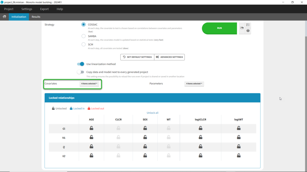
We can first try COSSAC. Because we’ve added log-transformed versions of CLCR and WT, e.g. we want to model a power-law relationship with these covariates, we can disable the non-logged version of these covariates in the covariates dropdown. It’s also possible to force or prohibit specific covariate-parameter relationships by using the lock icons to lock in or lock out specific relationships. Save as project_06, then click run to perform the search.

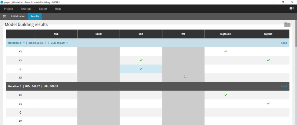
All the models tested are displayed with the best model listed first. Each model can be loaded by clicking on Load at the right. The folder with all models can be accessed by clicking “Open results folder” in the upper right. We see that the best model (Iteration 5) is an improvement over our last version from our manual covariate search (Iteration 1), which was used as a starting point (Δ-2LL=20 and ΔBICc=10). The best model added the covariate SEX to both V1 and Q compared to our last version with only logtCLCR on Cl and logtWT on V1. The search took 18 iterations in total. Differences between iterations are highlighted in blue.

SAMBA

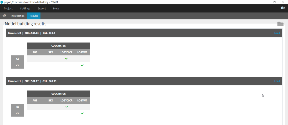
Next we can try SAMBA, which runs very quickly, so can be a good choice for a first approximation for models that take a long time to run. However, one limitation of SAMBA is that parameters without random effects are not included (Q and V2 in our case). Save the project as project_07 and run. Here we see that only two iterations were necessary, and the final model is the same as our final version with logtCLCR on Cl and logtWT on V1. While both iterations contain the same covariates, the likelihoods are slightly different (and an improvement over project_05) due to different parameter estimations influenced by different starting conditions.

SCM

Finally, we can try the SCM algorithm, the most exhaustive. Select SCM, and after verifying that the appropriate parameters and covariates are selected, save as project_08 and run (be aware this can take some time, ~15-30 min). In our case, the more exhaustive step-wise search performed by SCM took 42 iterations and resulted in the same model selected by COSSAC, that with logtCLCR on Cl,d logtWT on V1, and SEX on both V1 and Q.

Identification of the observation error model

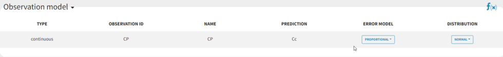
Until now, we have used the combined1 error model. The constant term “a” is estimated to be 0.027 in project_05, which is a little smaller than the smallest observation (around 0.1), and the RSE is estimated at 56%, meaning it is difficult to estimate. Thus it makes sense to try a model with a proportional error model only. We first create a project adding SEX as a covariate for both V1 and Q based on the covariate search, save it as project_09, and run it with the combined1 error model for comparison. The error model can be chosen in the “Statistical & Tasks” tab in the tab “Observation model” via the Error model drop down menu. We select proportional, save the project as project_10, and run the project.

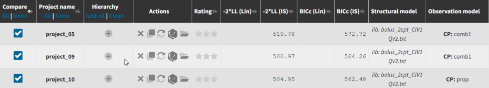
We can go back to Sycomore to compare the two error models. Under Hierarchy, click the button the the right of the directory name to rescan the directory. Now select project_05 (after manual covariate selection), project_09 (after additional covariates from automatic search), and project_10 (changing error model from combined1 to proportional). We see that adding the SEX covariate in project_6 improves the model fit (Δ-2LL=19 and ΔBICc=9), while changing to the proportional error model in project_10 increases -2LL by 4 but decreases BICc by 2 compared to project_06. Note that -2LL (as opposed to AIC) does not penalize for increased number of parameters, which BICc includes penalties for both the number of fixed and random effects estimated. Learn more about how Monolix estimates likelihood here.

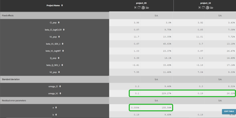
If we go to the comparison tab, we can see how the parameter estimates compare for the different error models. Importantly, we can see that the R.S.E., the relative standard error (standard error divided by the estimated parameter value), has decreased for omega_V1 and is no longer an issue for a with the proportional error model.

Convergence assessment

As a final check, we can do a convergence assessment, to verify that starting from different initial parameters or from different random number seeds leads to the same parameter estimates. Because Monolix will automatically generate ranges from which to sample the parameter bases on the initial estimates, we first click “Use last estimates: All” on the Initial estimates tab. Go back to Statistical model & Tasks and click on “Assessment” (below the run button), select 5 replicates with estimation of the standard errors and log-likelihood. To randomly pick initial values for all parameters, we select “All” under “sensitivity on initial parameters.” Monolix will automatically generate

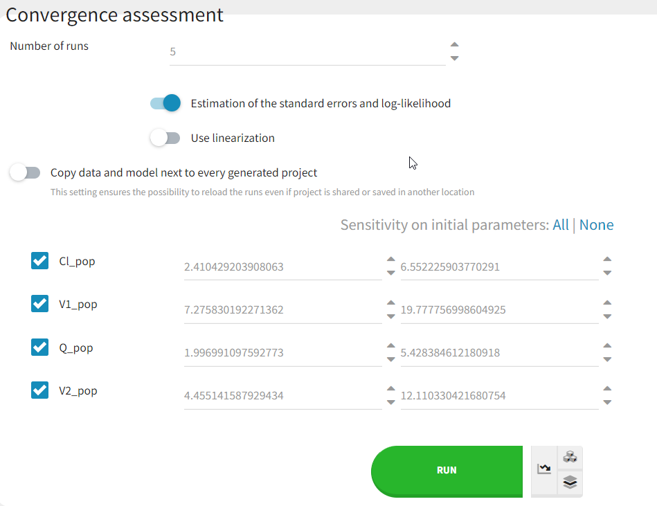
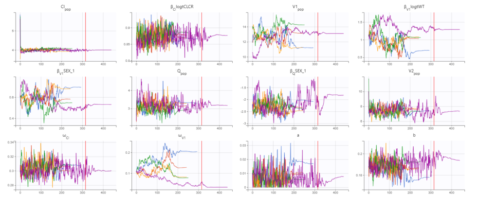
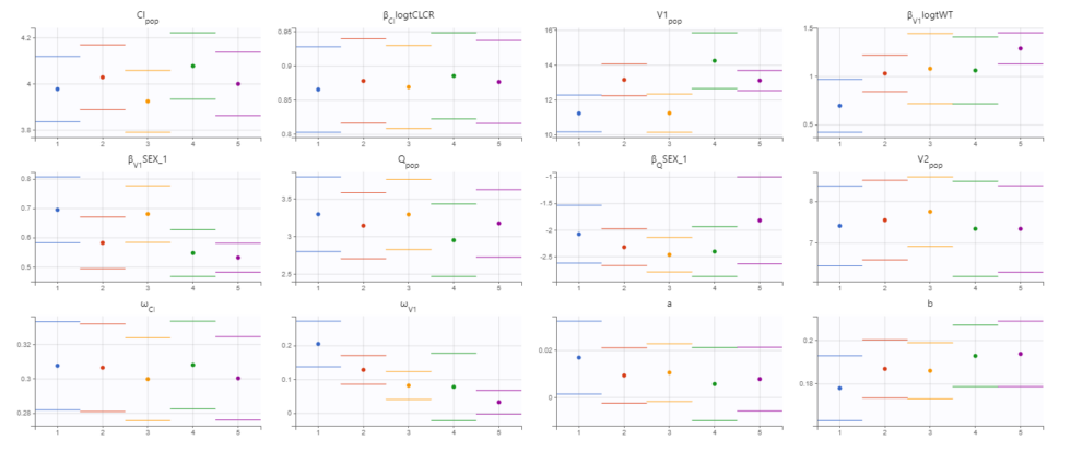
The displayed figures show a good convergence of all replicates to the same minimum. The first plot shows the evolution of the population parameter estimates over the iterations of the SAEM algorithm for each of the 5 replicates (Convergence indicator shown on second page). The second plot shows the final estimated parameter value (dot) and the standard errors (horizontal lines) for each parameter and each replicate (log-likelihood shown on second page) . The Fischer information matrix and importance sampling are also displayed. The estimated parameters and details of the individual runs can be found in the Assessment folder in the results folder. Note that the parameters related to V1 appear to be the most difficult to estimate and depend more on the starting conditions. This is likely due to the sparse nature of the data set, even though we have already removed random effect from V2 and Q.

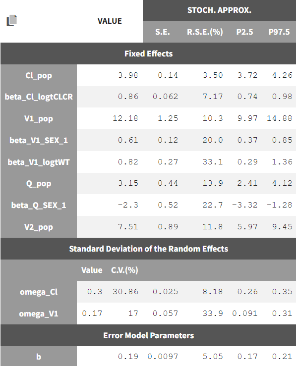
Final model summary

Our final model is the following:

• 2-compartment model, parameterized as (Cl, V1, Q, V2)

• the residual error model is proportional

• Cl and V1 have inter-individual variability, while Cl, V1, and Q have covariates

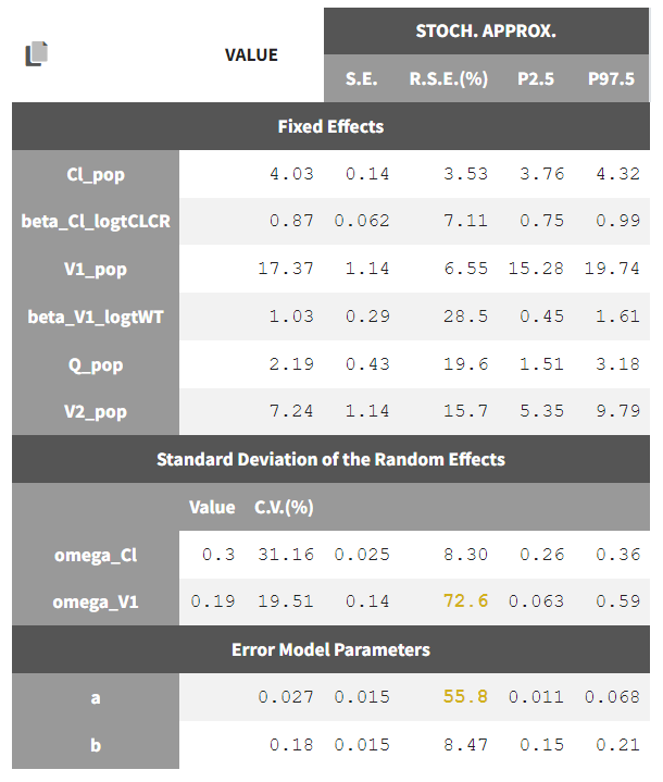
Theestimated parameters and their standard errors are:

Simulations for individualized dosing with Simulx and Monolix

A glance at Simulx possibilities

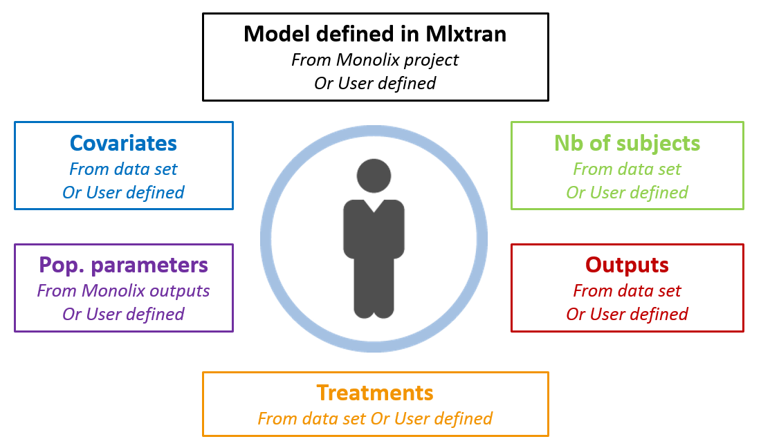
Now that we have a model, we can use it to do simulations. The saved Monolix project can be reused by Simulx for straightforward simulations. All project components (structural model, number of subjects, covariates, treatments, estimated parameter values and outputs) can either be reused from the project or data set, or be redefined by the user.

After opening a Simulx window, we can click on Import project and select the Monolix project file. This will automatically create the Simulx model, based on the structural and statistical model from the Monolix project. It will also automatically create elements that can be used for simulation, based on the results of the Monolix run.

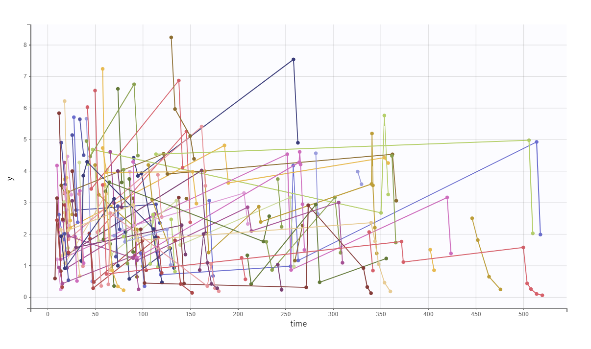
For example, if we just go to the Simulation tab and run the automatically defined simulation, we will resimulate the study with the same design (same group size, treatments, covariates, sampling points) using the estimated population parameters.

We obtain the following spaghetti plot, which is similar but different compared to the original data set:

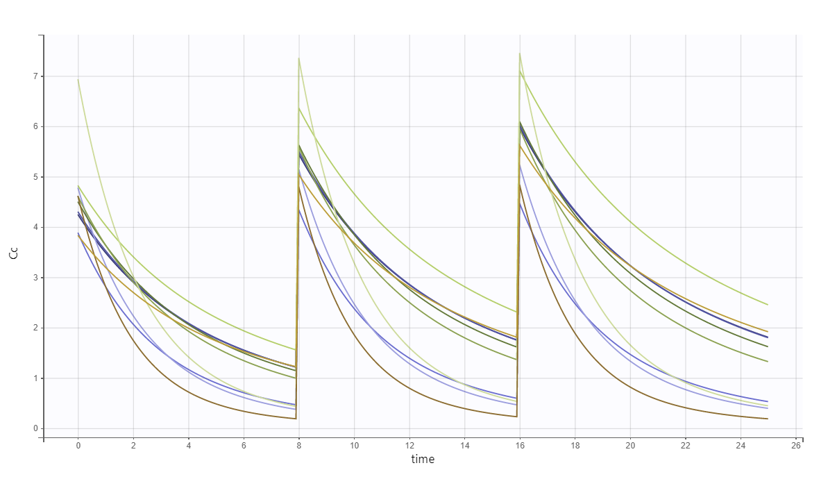
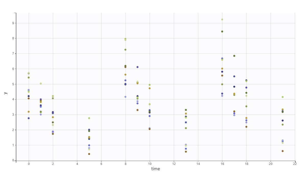
As a second example, we can:

• change the administration schedule to three doses of 80 mg at 0, 8 and 16 hr for all individuals,

• simulate only 10 individuals (resampled from the data set with their covariates),

• change the V_pop parameter to a higher value (while keeping the value estimated by Monolix for the other population parameters) and

• set denser measurement times.

The predicted exact concentrations and observed concentrations are the following, for the 10 simulated individuals:

Safety and efficacy with the usual treatment

In the present case, we are interested in optimizing the dosing regimen of Tobramycin. Usually Tobramycin is administrated as an intravenous bolus at 1 to 2 mg/kg every 8h (traditional dosing) or at 7 mg/kg once daily (new once-daily dosing). In this case study, we will start with the traditional dosing every 8h, at a dose of 1mg/kg. Higher clinical efficacy has been associated with peak drug concentration in the range 6-7 mg/L. Thus our efficacy target will be 6-7 mg/L for the Cmax, while the trough concentration must be below 2mg/L to avoid toxicity. What percentage of the population meets the efficacy and safety target, if Tobramycin is administrated according to the usual dosing regimen?

To answer this question, we will simulate the default treatment for the individuals of the data set. In the Monolix project, doses are given in mg. We now would like to work with doses in mg/kg, which means that we have to use the “Scale amount by a covariate” feature when creating treatments. We will get the weight information from the mlx_Cov covariate element (it contains the covariates from the data set) and use it to define the administration in a data frame listing the times and amounts for each individual. To simulate the steady-state peak and trough concentration for 1000 individuals, resampled from the data set, receiving 1 mg/kg every 8 hours, we:

• change the group size to 1000,

• define a new output element that outputs concentration between 280 and 295.9,

• define a new treatment element.

We can then see the concentration prediction interval:

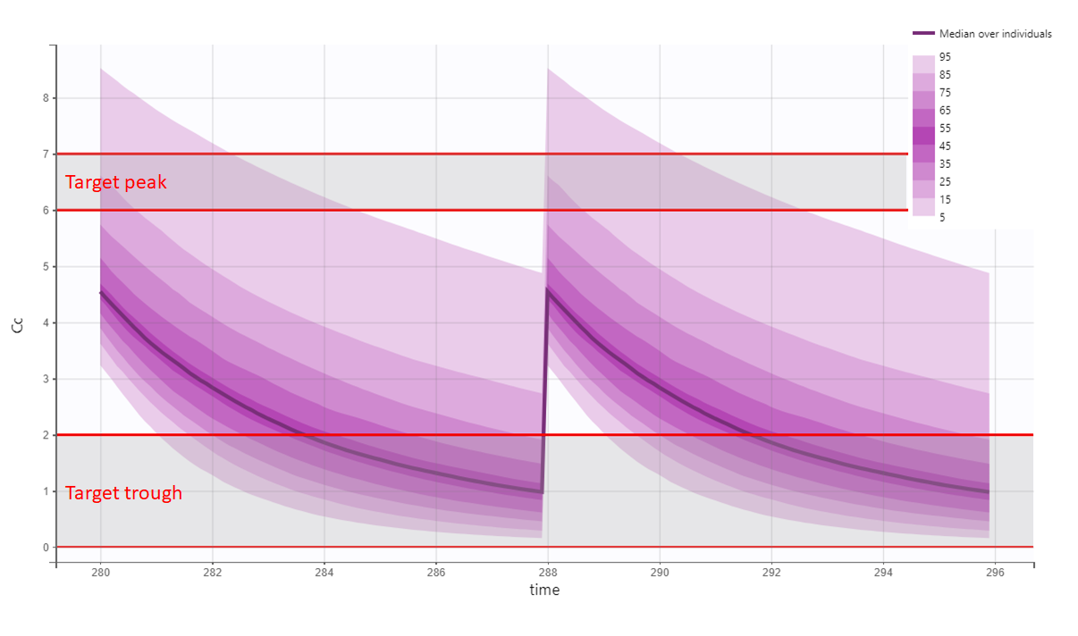
We see that a relatively large fraction of the individuals do not meet the safety criteria, the efficacy criteria or both. Using the simulation results and the outputs and endpoints feature, we can quantify the percentage of people meeting the criteria: with the default treatment, the chances that the treatment is effective are only 9% and the chances that the treatment is safe are 76%.

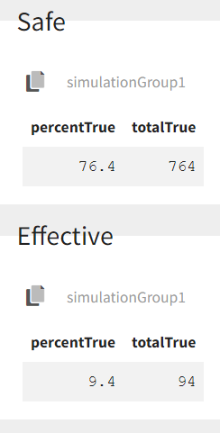
This calls for an individualization of the dose, to adapt the dosing regimen to the patients characteristics.

A priori determination of an appropriate dosing regimen for a specific individual

The poor performance of the default dosing prone us to adapt the dosing to the patients characteristics. To adapt the dosing, we can either use the patients covariates or try to get even more information of the patient using therapeutic drug monitoring.

Using the individuals covariates

We would like to a priori determine an appropriate dosing regimen for an individual, knowing its covariates values. For instance, we will consider an individual weighting 78 kg, with a creatinine clearance of 30 mL/min, which corresponds to a severe renal impairment. Knowing the covariates, we have an idea of the individual parameters for this individual, but uncertainty remains, which is captured in the random effects. For instance for the elimination rate k we have:

To determine a better dosing regimen than the default dosing for this individual, we will proceed in the following way:

1. consider a typical individual with weight 78 kg and creatinine clearance 30 mL/min

2. test if the efficacy and safety criteria are met with the default treatment. If not,

3. write an optimization algorithm to find a better dosing regimen

4. test the chances of the optimized dosing to be safe and efficient by considering the uncertainty of the parameters (i.e putting back the random effects)

We first consider a typical individual with this weight and creatinine clearance, i.e we neglect the random effects. How would the typical treatment perform on this individual? We simulate the patient in Simulx. This time, we do not take the covariates from the data set but define them ourselves and we use the mlx_Typical parameter element to simulate a typical individual.

# define project file
project.file <- '../monolixProjects/project_2cpt_final.mlxtran'

# an individual with WT=78 and CLCR=30
weight <- 78
clcr <- 30

# define output
outCc <- list(name = 'Cc', time = seq(279, 295.9, by=0.01))

# define covariates
covariates <- data.frame(id = 1, WT = weight, CLCR= clcr)

#disable random effects to simulate typical individual with this WT and CLCR
param=c(omega_k=0,omega_V=0) 

# define usual treatment
dosePerKg <- 1
interdoseinterval <- 8
adm <- list(time=seq(0,300,by=interdoseinterval), amount=dosePerKg*weight)

# run simulation of one individual 
res <- simulx(project = project.file,
 output = outCc,
 treatment = adm,
 parameter = list(covariates,param))

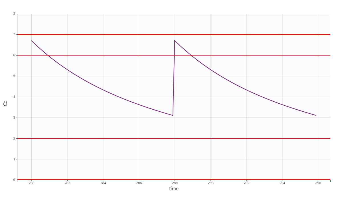
After plotting, we obtain the following figures that shows that for a typical individual with weight 78 kg and creatinine clearance 30 mL/min the trough concentration is too high so the default treatment has a high risk to be toxic.

We thus would like to adapt the dosing regimen for this individual, given its covariates values. We start by implementing a function using lixoftConnectors that returns the peak and trough concentrations at steady-state, for a given dose per kg and a given inter-dose interval:

getMinMax <- function(projectfile, dosePerKg, interdoseinterval, weight, clcr){
 
 outCc <- list(name = 'Cc', time = seq(35*interdoseinterval-0.05, 35*interdoseinterval+28, by=0.05))
 # define covariates
 covariates <- data.frame(id = 1, WT = weight, CLCR= clcr)
 
 # define treatment
 adm <- list(time=seq(0,38*interdoseinterval,by=interdoseinterval), amount=dosePerKg*weight)
 
 #disable random effects
 param=c(omega_k=0, omega_V=0)

 # run simulation of one individual
 N <- 1
 res <- simulx(project = projectfile,
 output = outCc,
 treatment = adm,
 parameter = list(covariates,param))
 
# set starting time to zero for easier comparison
 Conc <- res$Cc
 Conc$time <- Conc$time - Conc$time[1]

 maxi <- Conc[which(diff(sign(diff(Conc$Cc)))==-2)+1,]
 mini <- Conc[which(diff(sign(diff(Conc$Cc)))==2)+1,]

 result <- list(min=mini$Cc[1], max=maxi$Cc[1])
 return(result)
}

We then implement a simple optimization algorithm: if the peak is too high or too low, the dose is decreased or increased respectively. If the trough is too high, the inter-dose interval is increased. The code reads:

#initial dosing regimen
dosePerKg <- 1
interdoseinterval <- 8
weight <- 78
clcr <- 30
result <- getMinMax(project.file, dosePerKg, interdoseinterval, weight, clcr)

while(result$max < 6.3 | result$max > 6.7 | result$min> 1){
 if (result$max < 6.3 | result$max > 6.7){
 dosePerKg = dosePerKg + 0.2*(6.5-result$max)
 }else if(result$min > 1){
 interdoseinterval = interdoseinterval + 3
 }else{
 paste0("Error")
 }
 result <- getMinMax(project.file, dosePerKg, interdoseinterval, weight, clcr)
}

In the video below, one can visualize how the dose and the inter-dose interval evolve from the initial default treatment to a treatment achieving both efficacy and safety. For this individual, we propose 1.55 mg/kg administrated every 26 hr.

The proposed inter-dose interval may not be feasible in clinical practice. We can either take another close value, for instance 24h or modify the optimization algorithm to take into account the clinical practice constraints. In addition, instead of using a hand-made optimization algorithm, it is also possible to use more advanced algorithms implemented in separate R packages.

For the optimization above, we have considered a typical individual among the population of people with WT=78 and CLCR=30. We will now verify the chances of the optimized treatment to be safe and efficient, taking into account the uncertainty of the individual parameters for this individual, via the random effects.

The code is as follows. The only difference is that we do not disable the random effects anymore and simulate the individual 100 times to get a prediction distribution.

#output
outCc <- list(name = 'Cc', time = seq(35*interdoseinterval-0.05, 37*interdoseinterval-0.05, by=0.05))

# to get 
N <- 100

# define covariates
 covariates <- data.frame(id = 1, WT = weight, CLCR= clcr)

# define optimized treatment
adm <- list(time=seq(0,38*interdoseinterval,by=interdoseinterval), amount=dosePerKg*weight)

# run simulation of one individual, parameter k is drawn 
#from its distribution, taking into account the covariates
res <- simulx(project = project.file,
 output = outCc,
 treatment = adm,
 parameter = covariates)

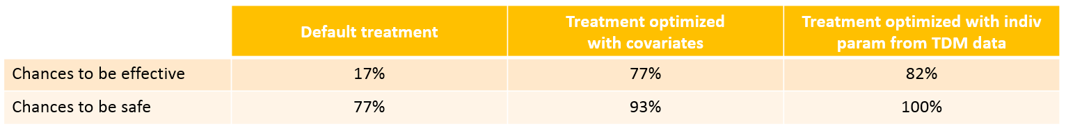
With the optimized treatment for this individual, there are 93% chances that the treatment is safe and 77% chances that it is effective. This is an improvement compared to the default treatment:

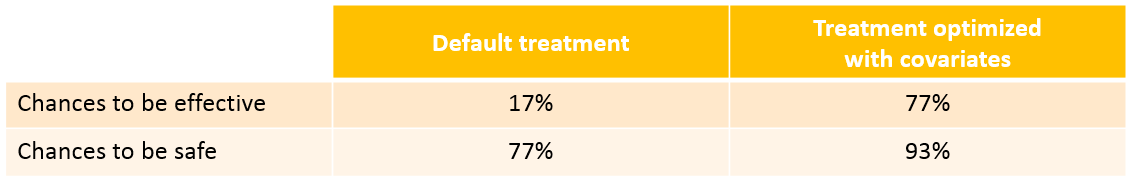
Yet if one would have a better estimate of the parameters for this individual instead of only its covariates information, one would be able to even better calibrate the dosing schedule. This is possible using therapeutic drug monitoring.

Using the individuals parameters, obtained from therapeutic drug monitoring (TDM)

After the first drug injection, it may be useful to monitor the drug concentration in order to adapt the subsequent doses. The goal is to use the measured concentrations to determine the parameters of this individual and use these estimated parameters to simulate the expected concentration range after several doses and adapt the dosing accordingly.

Let’s assume that for our individual (weight=78 kg, creatinine clearance=30 mL/min), we have started with the a priori proposed dose 93.6 mg, and have measured the concentration at a few time points after the first dose:

ID   TIME  DOSE     Y  WT  CLCR
1     0    93.6     .  78   30
1     1    .     3.59  78   30
1     3    .     2.75  78   30
1     5    .     2.07  78   30
1     8    .     1.11  78   30

We can use Monolix to estimate the individual parameters of this individual, fixing the population parameters to those estimated previously. In the monolix project below, the model is exactly the same as the final model determined using the clinical data set, the population parameters have been fixed to the estimated values and the data set has been replaced by the one above, recording the TDM measurements for this individual:

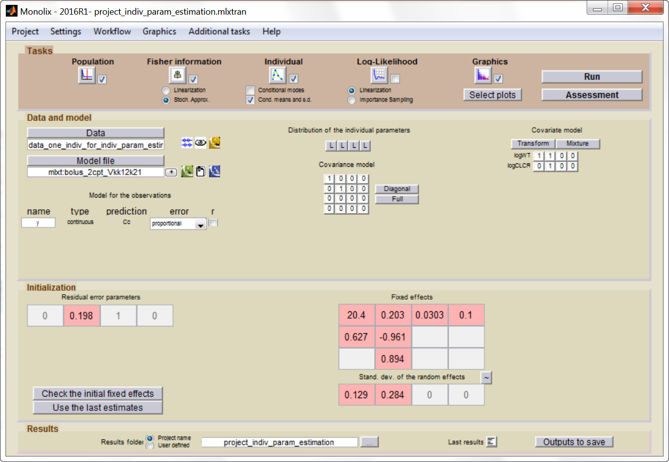
After having run the estimation of the
population parameters (which just prints the parameters to a file, as
all population parameters are fixed), we can estimate the mean, mode and std of the conditional distribution 
(individual button). The results are printed in the file
“indiv_parameters.txt” in the result folder. We obtained the following
values: k_mean=0.112, k_std=0.024, V_mean=23.8 and V_std=2.26.

The “IndividualFits” graphic shows the prediction using the estimated conditional mean and the drug monitoring data:

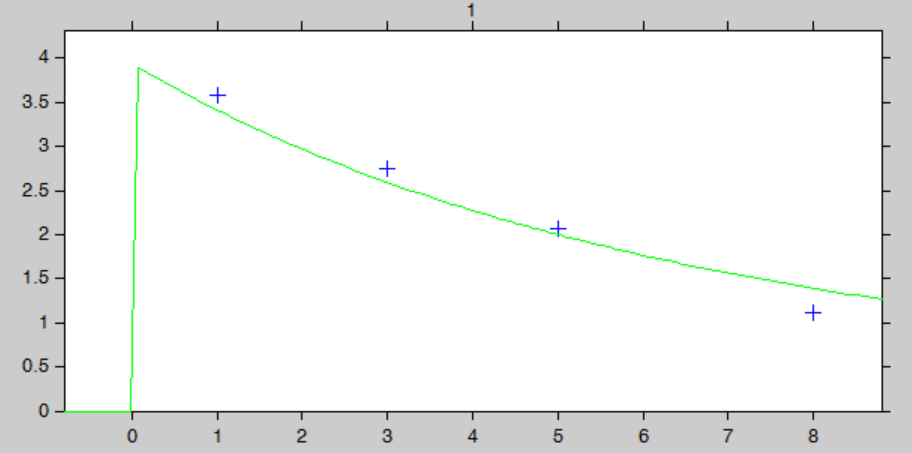
Click here to download the Monolix project to estimate the individual parameters.

We now would like to use the estimated individual parameters to adapt the treatment. In Simulx, it is not possible to directly set the value of the parameters at the individual level when using a project file as input. We will instead work with a model file as input, containing the structural model. In a very similar manner as previously, we define a getMinMax function (below) and an optimization loop. The parameters V, k, k12 and k21 are set to the mean of the conditional distribution calculated with Monolix.

getMinMax_withModel <- function(modelfile, dosePerKg,interdoseinterval, reference, weight,clcr){
 
 outCc <- list(name = 'Cc', time = seq(35*interdoseinterval-0.05, 35*interdoseinterval+28, by=0.05))
 
 # parameter values fixed
 parameters <- data.frame(id = 1, 
 V = 23.8,
 k = 0.112,
 k12 = 0.0303, 
 k21 = 0.1)
 
 # define treatment
 adm <- list(time=seq(0,38*interdoseinterval,by=interdoseinterval), amount=dosePerKg*weight)
 
 # run simulation of this individual
 res <- simulx(model = modelfile,
 output = outCc,
 treatment = adm,
 parameter = parameters)
 
 Conc <- res$Cc
 Conc$time <- Conc$time - Conc$time[1]

 maxi <- Conc[which(diff(sign(diff(Conc$Cc)))==-2)+1,]
 mini <- Conc[which(diff(sign(diff(Conc$Cc)))==2)+1,]

 result <- list(min=mini$Cc[1], max=maxi$Cc[1], ref=reference)
 return(result)
}

The optimization leads to the following schedule: 1.80 mg/kg every 26 hr.

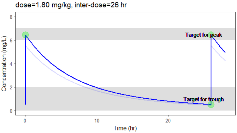
Due to the uncertainty in the individual parameters for this individual, there is also an uncertainty on the simulated concentration.

To verify the chances of the optimized treatment to be safe and efficient, we would like to take into account the distribution of the individual parameter instead of only the mean. The distribution of the individual parameters is a joint distribution (without analytical formula), that can for instance be estimated via a Monte-Carlo procedure. As Monolix does not permit to directly output the result of the Monte-Carlo procedure, we use the following trick: we can set the number of chains (i.e the number of times the data set is replicated) to a high number, which permit to simulate several times the same individual. This is done in Settings > Pop. parameters > nb chains. Then, in the covariates graphic, with the “simulated parameter” option, Monolix draws one parameter value from the conditional distribution per individual (so 1000 if one has used 1000 chains for instance). These values can be outputted to a file by going to Graphics > Export graphics data.

Click here to download the associated Monolix project

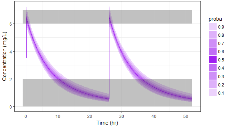
The values in the outputted file are thus draws from the joint conditional distribution and represent the uncertainty of the individual parameters. We can use them to simulate the prediction interval for the concentration.

N <- 1000

# load individual parameter values from covariates graphic
file.indiv.param <- '../monolixProjects/project_indiv_param_estimation_1000chains
                     /GraphicsData/Covariates/Covariates_Simul.txt'
data <- read.table(file.indiv.param, header = TRUE, stringsAsFactors = FALSE)

V_ind <- exp(data[data$Cov_WT==78,'Param_log.V.'])
k_ind <- exp(data[data$Cov_WT==78,'Param_log.k.'])

# parameter values
parameters <- data.frame(id  = (1:N),
                         V  = V_ind[1:N],
                         k  = k_ind[1:N],
                         k12 = 0.0303,
                         k21 = 0.1)

# run simulation of N individual, parameter k is drawn from its distribution
outparam <- c("V","k","k12","k21")
res2 <- simulx(model = structuralModelFile,
 output = list(outCc,outparam),
 treatment = adm,
 parameter = parameters)

# calculate the percentiles and plot
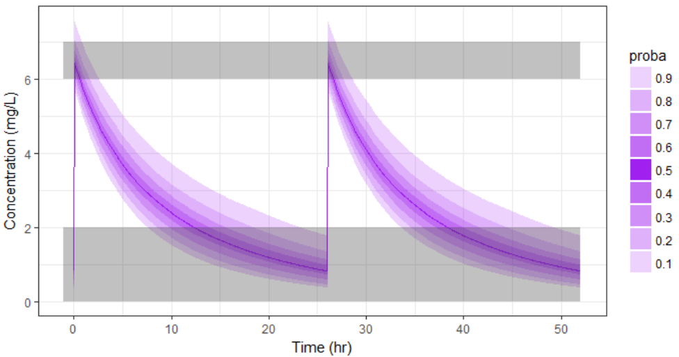
pPrct2 <- prctilemlx(res2$Cc, band=list(number=9,level=90)) +
 scale_x_continuous("Time (hr)") + 
 scale_y_continuous("Concentration (mg/L)") + ylim(c(0,7.5))

print(pPrct2)

With the newly optimized treatment, there are 82% chances that the treatment is effective and 100% chances that it is safe, which is an improvement compared to the treatment proposed using the covariates only.

A note on individual predictions for individualized dosing

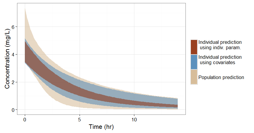
In the previous sections, we have seen three ways of predicting the concentration time course of an individual:

1. If no covariate information is available for this individual, we only know that the concentration time course for the individual will be within the prediction interval of the entire population, which is pretty large (tan color in the figure below).

2. If the covariates of this individual are available, we can use them to get a reduced distribution of the parameters k and V for this individual. The associated concentration prediction (bleu color in the figure) is narrower compared to the first case.

3. If in addition to the covariates, a few measures can be made (drug monitoring), the conditional distribution of parameters k and V (given theses measures and the previously estimated population parameters) can be obtained. This leads to an even more narrow concentration prediction interval (brown in the figure).

Note that for this figure we have used a more typical individual without renal impairment (CLCR=80 mL/min).

Conclusion

This example shows how a  personalized treatment can be proposed using population PK modeling and simulation, and how the MonolixSuite software components facilitate an efficient implementation. The modeling/simulation approach permits to precisely assess the trade-off between the prediction precision and the costs of information acquisition. Covariates are usually relatively cheap to measure but in the present case lead to only a moderate reduction of the prediction interval. On the other hand, therapeutic drug monitoring is more expensive but permits a strong narrowing of the concentration prediction interval, which in turn permits a better determination of an effective and safe dosing regimen.