Guide: From NONMEM to Monolix

Welcome to Monolix! This guide is designed as a detailed reference for pharmacometricians transitioning from NONMEM. Instead of a linear walkthrough, this document is structured by topic, allowing you to look up a specific part of a NONMEM control stream (e.g., $OMEGA, $DES) and find its direct equivalent and implementation details in Monolix.

Our goal is to provide a comprehensive map from the NONMEM syntax you know to the integrated, graphical workflow of Monolix.

1. The Dataset ($INPUT)

The foundation of any model is the dataset. While NONMEM uses the $INPUT block with fixed column names, Monolix uses a flexible column tagging system. You can find detailed instructions on how to load a dataset in Monolix here.

Basic Column Mapping

When you load a dataset in Monolix, you assign a functional type to each column.

You can find more information about all the column types available in Monolix here.

The CMT Column

The CMT column in NONMEM is often used for multiple purposes. Monolix separates these functions for clarity:

• To distinguish different observation types (e.g., CMT=2 for PK, CMT=3 for a PD biomarker): Tag the CMT column as OBSERVATION ID.

• To direct doses to different compartments (e.g., CMT=1 for IV, CMT=2 for oral): Tag the CMT column as ADMINISTRATION ID.

• If CMT is used for both: You must split it into two separate columns in your dataset before loading it into Monolix—one for observation types and one for administration types.

BLQ Data

Handling data below the limit of quantification (BLQ) is vastly simplified.

• In NONMEM: You must implement the M3/M4 method manually with complex IF/THEN logic in the $ERROR block to calculate the likelihood of an observation being censored.

• In Monolix: The process is entirely graphical:

  1. Create a flag column in your dataset (e.g., BLQ) with 1 for censored observations and 0 for non-censored.

  2. In the rows where BLQ=1, set the DV column to the value of the limit of quantification (LOQ).

  3. In the Monolix Data tab, tag your BLQ column as Censoring.

• M3 vs. M4 Method: Monolix automatically selects the method. If you provide a LIMIT column in your dataset where the value is 0 for censored data, the M4 method is used. Otherwise, the M3 method is used by default.

Filtering Data ($IGNORE)

To replicate NONMEM's $IGNORE statement, use the Filter feature in the Monolix Data tab. You can build complex rules to exclude individuals or specific records (e.g., DOSE == 0 to exclude a placebo arm).

Example:

NONMEM	Monolix
CODE IGNORE=(DOSEMG.EQ.0)

Time-Varying Covariates (Regressors)

There is a critical difference in how time-varying covariates are handled between data points:

• NONMEM: Uses "next value carried backward."

• Monolix: Uses "last observation carried forward" by default. You can also select "linear interpolation" as an alternative method in the data formatting options. If the exact timing of a covariate's effect is critical, you may need to shift the values in your regressor column by one row in the dataset to achieve the same behavior as in NONMEM.

2. The Structural Model ($PK, $DES)

This is where you define your model's equations. In Monolix, this is done in the model file, written in the MLXTRAN language. How to choose a model file in Monolix is explained here.

Using the Library ($SUBROUTINES)

The easiest approach is to select a model from Monolix's extensive library. This is the equivalent of using an ADVAN routine and is the recommended starting point. The library contains validated models for PK, PD, TMDD, TTE, and more.

Example:

Writing Custom Models Using ODEs

ODE Systems (from $DES)

You can often copy-paste your NONMEM ODEs into the EQUATION section of a model file with minor syntax changes.

IF (TIME.GT.0) INH = (IMAX*FLC)/(IC50+FLC)

IF t>0
  INH = (IMAX*FLC)/(IC50+FLC)
END

ODE Solver Settings

To control the ODE solver (equivalent to $ADVAN... TOL=...), you can add keywords to the EQUATION section of your model file:

• Solver Type: odeType = stiff forces the use of a stiff solver, equivalent to $ADVAN13. The default is a non-stiff solver.

• Solver Tolerance: You can adjust the relative and absolute tolerance:

  • odeRelTol = 1e-6 (this is the default value)

  • odeAbsTol = 1e-9 (this is the default value)

Example:

Dosing and Model Inputs (depot() macro)

The depot() macro is a powerful tool that replaces much of the logic from $PK or $MODEL. It links doses from the dataset to your model variables. You can find all the options available when using the depot macro here.

; This single line handles an oral dose with a lag time,
; bioavailability and first order absorption
depot(target=Aa, Tlag=Tlag, p=F, ka=ka)

This is far more explicit and readable than NONMEM's implicit compartment-based dosing.

Compartment Definitions

Parts of the NONMEM control stream that define compartments and look like this can be completely omitted from the Monolix structural model:

$MODEL
COMP = (DEPOT, DEFDOSE)
COMP = (TDA)

Transit Compartments

This is a prime example of Monolix's simplification:

; Ktr = transit rate, Mtt = mean transit time
depot(target=Ac, Ktr, Mtt)

Model Outputs and Error Logic (from $ERROR)

The complex logic in a NONMEM $ERROR block is split into two clear parts in Monolix:

1. Defining Outputs: You declare your model outputs in the OUTPUT section of the MLXTRAN file:

   CODE

   OUTPUT:
   output = {Cc, E}

2. Mapping Outputs: In the GUI, you graphically map each model output to its corresponding OBSERVATION ID. This completely replaces the need for IF (CMT.EQ.2) THEN ... statements. Residuals (RES, WRES) are calculated automatically and do not need to be coded.

3. The Statistical Model: ($THETA, $OMEGA, $SIGMA, Covariates)

This is where the Monolix workflow differs most from NONMEM. All aspects of the statistical model are defined visually in the Statistical Model & Tasks tab.

Model Parameters ($THETA, $OMEGA, $SIGMA)

Fixed Effects ($THETA)

These are the population typical values (_pop) for each parameter in your model (e.g., V_pop, Cl_pop). They are defined in the input section of the structural model file.

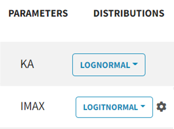
Random Effects ($OMEGA)

To add inter-individual variability (an ETA), simply check the Random Effect box for a parameter. Select the parameter distribution from the dropdown menu (choose between lognormal, normal and logitnormal).

NONMEM	Monolix
CODE TVKA = THETA(1) KA = TVKA*EXP(ETA(1)) PHI = THETA(12) + ETA(10) IMAX = EXP(PHI)/(1+EXP(PHI))

If the parameter distribution is not available (e.g., proportional or Box-Cox distribution), it has to be implemented by separating fixed and random effects:

CL = THETA(3) * (1 + ETA(3)

[LONGITUDINAL]
input = {CLpop, etaCL, …}

EQUATION:
CL = CLpop * (1 + etaCL)

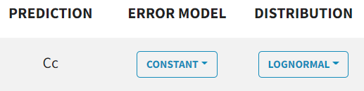
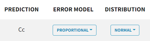
Residual Error ($SIGMA)

The $ERROR block's error definition is replaced by a dropdown menu for each observation type, where you can select proportional, constant, combined1, combined2.

Examples:

NONMEM	Monolix
CODE $ERROR Y = SQRT(ADD**2 + (PROP*IPRED)**
CODE $ERROR IPRED=LOG(F) Y=IPRED+ERR(1)

Covariate Models

How you translate a continuous covariate relationship depends on the mathematical form.

Categorical covariates

Monolix simplifies the implementation of categorical covariates by replacing NONMEM's manual IF/THEN logic with a graphical approach.

In NONMEM, you typically code the effect of a categorical covariate explicitly:

IF (SEX.EQ.0) THEN 
  TVCL = THETA(1) 
ELSE 
  TVCL = THETA(2) 
ENDIF

Or, for a multiplicative effect on a log-normal parameter: TVCL = THETA(1) * THETA(2)**SEX.

The translation in Monolix involves two simple steps:

1. Tag the Covariate: In the Data tab, identify your categorical variable column (e.g., SEX) and tag it as a CATEGORICAL COVARIATE. Monolix will automatically detect the different categories (e.g., 0 and 1, or F and M).

2. Add the Effect: In the Statistical Model tab, select the parameter you want the covariate to act on (e.g., Cl). Click to add SEX as a covariate.

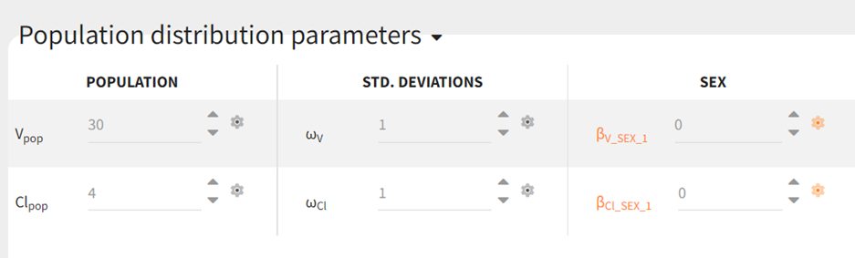
Monolix automatically estimates a typical value (_pop parameter) for the reference category and a beta coefficient for the effect of each other category.

For example, the NONMEM code TVCL = THETA(1) * THETA(2)**SEX is equivalent to the Monolix formula:

Here, corresponds to THETA(1) (the typical clearance for the reference category, SEX=0), and corresponds to log(THETA(2)) (the log of the multiplicative factor for SEX=1). You don't need to write this equation; Monolix builds it for you.

Continuous Covariates - Exponential Relationship

This is the default for log-normally distributed parameters in Monolix and is the most common case.

• Formula:

• NONMEM Equivalent: TVCL = THETA(1) * EXP(THETA(2)*WT)

• How to implement: Simply add the covariate to the parameter in the GUI by selecting the checkbox under WT and next to Cl in the Statistical model & Tasks tab. Monolix defaults to this linear relationship on the log-transformed parameter.

Continuous Covariates - Power-Law Relationship

This is another common case.

• Formula:

• NONMEM Equivalent: TVCL = THETA(1) * (WT/70)**THETA(2)

• How to implement:

  1. Click on the name of the covariate WT in the Statistical model & Tasks tab and then select “Add log-transformed”.

  2. Covariate logtWT will appear. Monolix will normalize the covariate when transforming using the weighted mean of the dataset values of that covariate. If you want to change the value by which the covariate is normalized, you can click on the name of the covariate and select “Edit”.

  3. You can add the covariate by clicking on the checkbox next to Cl and under logtWT. Adding a log-transformed covariate is equivalent to using the power-law relationship for the covariate effect:

Other Relationships

For any relationship that cannot be built in the GUI (e.g., a sigmoid Emax model, a time-varying covariate effect), you must implement it directly in the structural model file.

1. Tag the covariate as a REGRESSOR in the Data tab. This makes its value available at each time point within the model.

2. Implement the formula in the MLXTRAN code. List the regressor as an input and write the custom equation.

   CODE

   [LONGITUDINAL]
   input = {Cl_pop, ..., mycov}
   mycov = {use=regressor}
   
   EQUATION:
   ; Custom relationship implemented directly
   tvCl = Cl_pop * (1 + (Emax * mycov) / (EC50 + mycov)) 
   ...

More detailed information about custom covariate-parameter relationships: Complex covariate-parameter relationships.

Inter-Occasion Variability (IOV)

4. Initial Estimates and Estimation

Setting initial estimates requires careful attention to the differences in statistical definitions between the two platforms.

Fixed Effects ($THETA)

These are generally straightforward. Enter the THETA values as initial estimates for the _pop parameters. Be careful with transformations. For a NONMEM covariate model like TVCL = THETA(1) * THETA(2)**SEX, the corresponding Monolix parameter beta_Cl_SEX is actually log(THETA(2)). So if THETA(2)=1, beta_Cl_SEX=0.

Random Effects ($OMEGA and $SIGMA)

• Variance vs. Standard Deviation: NONMEM's $OMEGA and $SIGMA blocks define variances. Monolix works with standard deviations. To convert, use the formula:

• Covariance vs. Correlation: NONMEM's $BLOCK statement defines covariances. Monolix uses correlation coefficients (rho), a value between -1 and 1. To convert, use the formula:

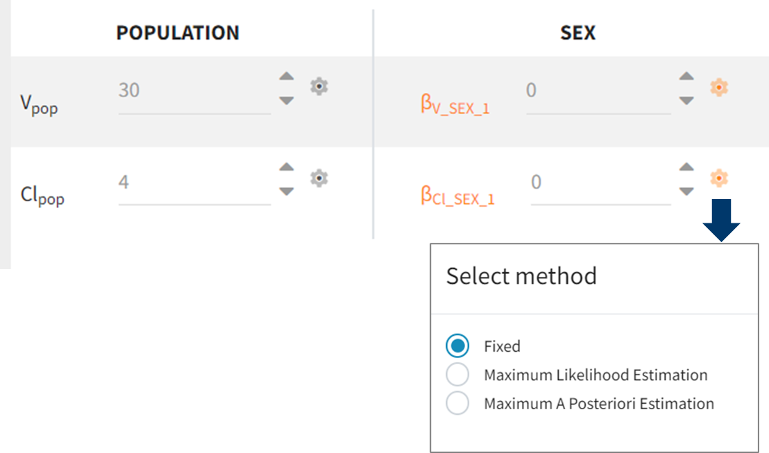
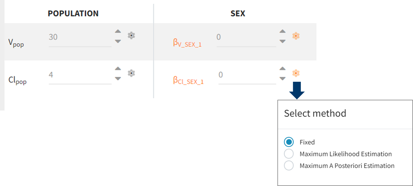
Fixed Parameters

In Monolix, parameters are fixed in the Initial estimates tab by clicking on the gear icon next to initial estimates and selecting “Fixed”.

NONMEM	Monolix
CODE $THETA (0.0,4) ;[CL] (0.0,30) ;[V] (0.75 FIXED) ;[CL~WT] (1.0 FIXED) ;[V~WT]

Running the Model and Related Tasks

The $ESTIMATION, $COVARIANCE, and $TABLE records are replaced by a graphical task manager in Monolix, which offers a more comprehensive and integrated set of tools.

• Population Parameters: This is the main estimation task, equivalent to $ESTIMATION. It uses the SAEM algorithm to find the maximum likelihood estimates of the population parameters.

• Individual Parameters (EBEs): This task calculates the Empirical Bayes Estimates (EBEs) of the parameters for each individual, along with the conditional standard deviations.

• Standard Errors: This is the equivalent of $COVARIANCE. It calculates the standard errors (and RSE%) for the population parameters by computing the Fisher Information Matrix.

• Likelihood: This task computes the log-likelihood of the model, equivalent to the final objective function value in NONMEM. It can be calculated via the more accurate (but slower) Importance Sampling or the faster Linearization method.

• Plots: This task automatically generates a full suite of diagnostic plots (VPCs, individual fits, observation vs. prediction, residual plots, etc.), replacing the need for external tools like PsN and Xpose.

• Integrated Tools: Monolix also includes built-in tools for tasks that require third-party software in the NONMEM world, such as Bootstrap for confidence intervals and Stepwise Covariate Modeling (SCM) for automated covariate searches.

Good luck, and welcome to the MonolixSuite!

Webinar

Here you can take a look at our webinar on this topic:

https://www.youtube.com/watch?v=PUCanvv5s0o&pp=ygURbm9ubWVtIHRvIG1vbm9saXg%3D

Here you can download the examples from the webinar: