Outputs of simulations are variables from the longitudinal model of continuous, discrete or event type. There are two outputs groups:
-
Main outputs
-
Model predictions defined in the structural model as the “output” (eg. Cc).
-
Observations (model predictions with an error model) defined in the observation model (eg. y1).
-
All variables defined in the structural model as “tables” (eg. AUC).
-
-
Intermediate outputs
-
Variables computed in the structural model and not listed as an “output” or “table” in the OUTPUT block (eg. amount in the peripheral compartment, time varying clearance).
-
Regressors.
-
Variables defined with the “additional lines” in the model definition.
-
Loading a model automatically generates the “main outputs”. Model predictions and tables are on a default time grid. If a project is built from scratch, then model observations use also the default time grid. Otherwise, in case of project imported from Monolix, they are on a grid given by the measurement times from the Monolix dataset.
Demos: 3.5.outputs, 7.noncontinuous_outputs
New output element
Outputs correspond to output variables, which can be written or selected from the list (green frame).
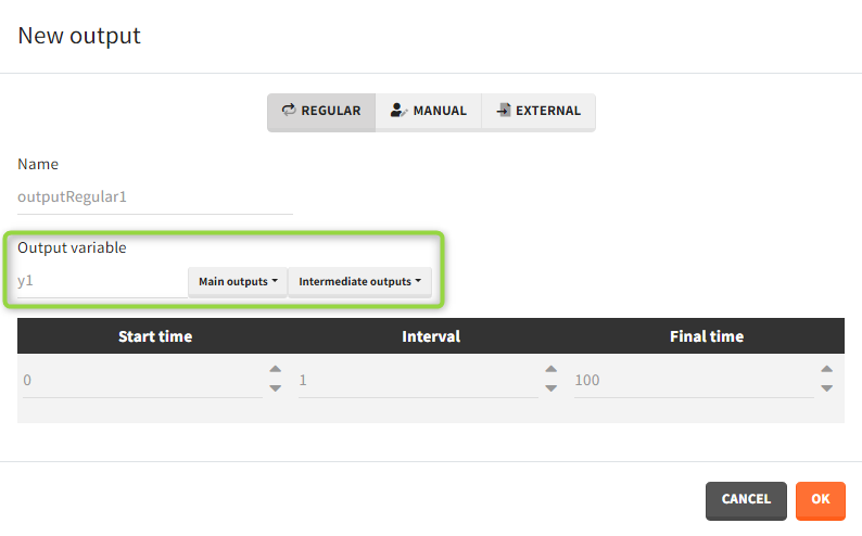
It is possible to have different outputs of the same variable. For example, one output shows the time evolution over a treatment period and another gives a value at the end of treatment to define an endpoint. However, charts display these outputs on one plot with merged time grids.
There are three output types.
-
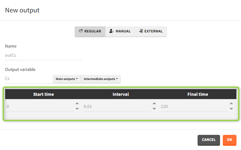
Regular: It is a vector on a regular time grid (start time, step, final time, (occ)) common for all subjects.
-
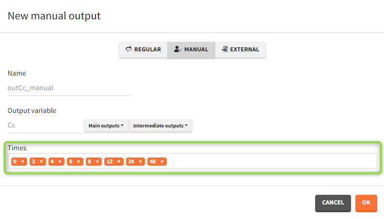
Manual: It is a vector with manually defined list of time points (use “space” to separate them) common for all subjects.
-
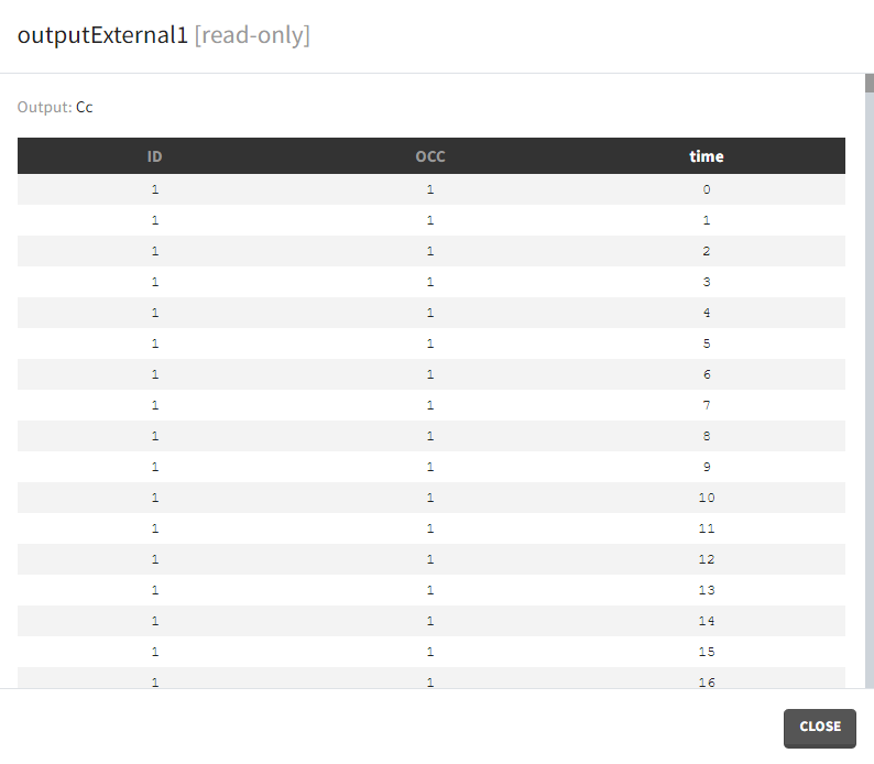
External: It is a file with a table that has: a mandatory column “time” for time points, an optional column “id” (in the absence of the “id” column the time grid is equal for all subjects), and an optional column “occ” for occasions.
Occasions
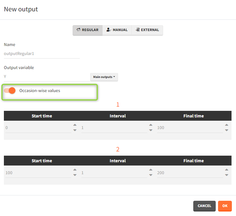
By default, the regular and manual output types apply to all subject-occasions. If occasions are common among all individuals, then an option “occasion-wise values” is available. In this case each occasion has a separate time grid.
Time-to-event outputs
Time limits (start time and final time) define the observation period during which the survival curve is computed. The final time thus defines the censoring time. Intermediate times are ignored. The time grid must be the same for all individuals. If an external file is provided with different start and end values for each individual, the events will be simulated on the same observation period for all individuals, using the min(start time) and max(end time) over all individuals.
Outputs imported from Monolix
Importing a Monolix project generates automatically output elements for the “main output” variables.
-
mlx_observationName (eg. mlx_y1, mlx_y2): For each output of the observation model it is a table with ids and observation times corresponding to the measurements read from the dataset.
-
mlx_predictionName (eg. mlx_Cc, mlx_R): For each continuous output of the structural model it is a vector with a uniform time grid with 250 points on the same time interval as the observations.
-
mlx_TableName: For each variable of the structural model defined as table in the OUTPUT section it is a vector with a uniform time grid with 250 points on the same time interval as the observations.

