Reference-scaled average bioequivalence - FDA approach (RSABE - high variable drugs)

The FDA implements reference-scaling as RSABE, Reference-Scaled Average Bioequivalence. Like EMA's ABEL it starts from ordinary average bioequivalence, but rather than widen the limits and re-run the 90% CI test, it replaces that test with one linearized criterion: the squared mean difference between products, penalised by the reference variability, must have a 95% upper confidence bound at or below zero. The more variable the reference, the easier this is to satisfy, the same "the more variability, the wider the margin" idea as ABEL, only written as a single inequality rather than a moving acceptance interval. A separate point-estimate constraint on the geometric mean ratio (GMR) keeps the two products from differing too much on average.

Unlike the EMA method, FDA reference-scaling applies to both AUC and Cmax (each parameter switches on its own variability), and there is no upper cap on how far the criterion relaxes.

The FDA guidance defines two reference-scaling methods. This page documents the one for highly variable drugs (HV), the widening RSABE from the Progesterone guidance. The second method, for narrow therapeutic index (NTI) drugs, scales in the opposite direction (limits narrow as the reference becomes less variable) and adds a variability-comparison test; it is
not implemented in this script. See HV vs NTI below.

Concept and mathematics

RSABE keeps the same raw inputs as any BE analysis, the test-vs-reference mean difference and the reference variability, but combines them into one criterion rather than a CI-in-interval check. The analysis has four steps:

1. Within-reference variability

The FDA estimates the within-reference variance by the method of moments from the reference replicates. For each subject the two reference measurements give a contrast (natural-log scale); an ANOVA of on sequence has residual mean square equal to twice the within-reference variance, so

where represents the residual (error) mean square. This needs the reference given at least twice per subject, which is why a replicate design is required. A pooled within-subject CV from a standard BE ANOVA (test and reference together) is not

2. Deciding whether to scale

Each parameter is tested by reference-scaling only if the reference is highly variable; otherwise it falls back to conventional unscaled ABE:

The threshold = 0.294 corresponds to ≈ 30%. Because AUC and Cmax each carry their own one parameter can be scaled while the other is not.

3. The reference scaled criterion (Howe’s Approximation I)

With the regulatory constant and

the null hypothesis of inequivalence is:

Meaning that non-equivalence is assumed by default: the squared gap between the product means is taken to exceed the variability-scaled allowance and bioequivalence is concluded only when the data are strong enough to reject this.

Reference-scaling widens the acceptance region because the penalty term grows with the reference variability. Rearranged, the pass condition is:

so a more variable reference tolerates a larger mean difference. Its two terms (squred means and scaled variance) follow different sampling distributions, so each is estimated and bounded separately and then combined into a single upper confidence bound by Howe's Approximation I [1].

Here LCL/UCL are the 90% confidence limits of the T-vs-R mean difference and is the degrees of freedom of the -contrast ANOVA. is the (approximate) 95% upper confidence bound of the criterion, and the scaled test passes when

4. The point-estimate (GMR) constraint

In every case the GMR must also lie within the fixed interval so however variable the reference, the products' averages can never fall outside the usual 80-125% limits. For a scaled parameter the decision is and the GMR constraint; for an unscaled parameter it is the 90% CI inside 80.00-125.00% (which already implies the GMR constraint).

Implied limits

When a parameter is scaled, there's no fixed 80-125% interval to check the CI against anymore. The decision is a formula (the criterion ), not an interval, but it can be back-translated into an implied limit for interpretation, using

These implied limits widen without bound as grows. They are shown in the report for readability; the formal decision remains

HV vs NTI

The FDA guidance defines two reference-scaling methods. Both use the same criterion and 95% upper-bound test described above; they differ only in their constants and purpose:

• Highly variable (HV) drugs: the script below. = 0.25, switch at = 0.294 ( ≈ 30%), limits widen with variability. Applies to AUC and Cmax.

• Narrow therapeutic index (NTI) drugs: not implemented here. = 0.10, so scaling makes the limits narrower as the reference becomes less variable, and it adds an explicit variability-comparison test (the upper 90% bound of must not exceed 2.5), run alongside the scaled ABE and an unscaled 80-125% check. A fully-replicate design (T and R each twice) is required.

Example

NCA parameters are computed in PKanalix; the reference-scaling is done in R via
lixoftConnectors. The example uses the PKanalix demo project project_repeated_4periods.pkx
(a full replicate design, TRTR/RTRT).

rm(list = ls())
path.prog <- dirname(rstudioapi::getSourceEditorContext()$path)

library(lixoftConnectors)
initializeLixoftConnectors(software = "pkanalix", force = TRUE)
library(dplyr)
library(flextable)
##############################################################################
loadProject(file.path(dirname(path.prog), "project_repeated_4periods.pkx"))
runNCAEstimation()

# Regulatory constants
sig0  <- 0.25                    # sigma_w0
theta <- (log(1.25) / sig0)^2    # 0.7967
k     <- log(1.25) / sig0        # 0.8926  (for implied-limits display only)
sWRsw <- 0.294                   # switching sWR (CVwR ~ 30%)
pe_lo <- 0.80; pe_hi <- 1.25     # point-estimate (GMR) constraint

# Read design + individual NCA values from project
set     <- getBioequivalenceSettings()
params  <- set$computedbioequivalenceparameters$parameters
seqc    <- set$linearmodelfactors$sequence
form    <- set$linearmodelfactors$formulation
ref     <- set$linearmodelfactors$reference
occ     <- getData()$header[getData()$headerTypes == "occ"]

nca_ind <- getNCAIndividualParameters()$parameters
test    <- setdiff(unique(nca_ind[[form]]), ref)[1]        # non-reference formulation
indiv   <- nca_ind %>% select(id, all_of(occ), all_of(seqc), all_of(form), all_of(params))

##############################################################################
# FDA RSABE for one PK parameter 
fda_rsabe <- function(p) {
  # per-subject intra-subject contrasts (natural-log scale)
  con <- do.call(rbind, lapply(split(indiv, indiv$id), function(d) {
    d  <- d[order(d[[occ]]), ]
    Tv <- log(d[[p]][d[[form]] == test])
    Rv <- log(d[[p]][d[[form]] == ref])
    data.frame(
      seq  = as.character(d[[seqc]][1]),
      ilat = if (length(Tv) >= 1 && length(Rv) >= 1) mean(Tv) - mean(Rv) else NA_real_,   # I = T - R
      dlat = if (length(Rv) >= 2) Rv[1] - Rv[2] else NA_real_)                            # D = R1 - R2
  }))

  # I contrast -> GMR + 90% CI (alpha = 0.10), x = est^2 - se^2, boundx
  di  <- con[!is.na(con$ilat), ]
  sf  <- factor(di$seq)
  fi  <- lm(ilat ~ 0 + sf, data = di)            # cell means per sequence
  mi  <- coef(fi); ng <- as.numeric(table(sf))
  w   <- rep(1 / length(mi), length(mi))         # equal-weight 
  est <- sum(w * mi)
  se  <- sqrt(summary(fi)$sigma^2 * sum(w^2 / ng))
  tc  <- qt(0.95, df.residual(fi))
  LCL <- est - tc * se; UCL <- est + tc * se
  pe  <- exp(est); x <- est^2 - se^2; boundx <- max(abs(LCL), abs(UCL))^2

  # D contrast -> s2wr (method of moments), dfd
  dd   <- con[!is.na(con$dlat), ]
  fd   <- lm(dlat ~ factor(seq), data = dd)
  s2wr <- summary(fd)$sigma^2 / 2; dfd <- df.residual(fd); sWR <- sqrt(s2wr)

  # linearized criterion (Howe's Approximation I)
  y      <- -theta * s2wr
  boundy <- y * dfd / qchisq(0.95, dfd)
  crit   <- (x + y) + sqrt((boundx - x)^2 + (boundy - y)^2)

  scaled <- sWR >= sWRsw
  PEok   <- pe >= pe_lo & pe <= pe_hi
  pass   <- if (scaled) (crit <= 0) & PEok else (exp(LCL) >= pe_lo & exp(UCL) <= pe_hi)

  # limits column: implied scaled limits when scaling, else the fixed 80-125
  lim <- if (scaled) exp(c(-1, 1) * k * sWR) else c(pe_lo, pe_hi)

  data.frame(
    Parameter = p, sWR = sWR, CVwR = sqrt(exp(s2wr) - 1),
    GMR = pe, CI_lo = exp(LCL), CI_hi = exp(UCL),
    lim_lo = lim[1], lim_hi = lim[2], critbound = crit,
    rule = if (scaled) "reference-scaled (sWR>=0.294)" else "unscaled ABE (sWR<0.294)",
    PASS = pass, stringsAsFactors = FALSE)
}

res <- do.call(rbind, lapply(params, fda_rsabe))

# For scaled params: decision is critbound <= 0 (Lower/Upper are IMPLIED limits, shown for interpretation only)
# For unscaled params: decision is 90% CI within 80.00-125.00%.
report <- with(res, data.frame(
  Parameter     = Parameter,
  Rule          = rule,
  `CVwR(%)`     = round(100 * CVwR, 2),
  sWR           = round(sWR, 4),
  `GMR(%)`      = round(100 * GMR, 2),
  `CI90_lo(%)`  = round(100 * CI_lo, 2),
  `CI90_hi(%)`  = round(100 * CI_hi, 2),
  `Lower(%)`    = round(100 * lim_lo, 2),
  `Upper(%)`    = round(100 * lim_hi, 2),
  critbound     = round(critbound, 4),
  BE            = ifelse(PASS, "PASS", "FAIL"),
  check.names   = FALSE, stringsAsFactors = FALSE))

print(report, row.names = FALSE)
flextable(report) %>% autofit()

How the script works. The steps correspond to the four-step concept above; each PK parameter is processed independently by fda_rsabe():

• Design is read, not hardcoded. getBioequivalenceSettings() returns the parameter list and the column names, the only study-specific input is the .pkx path; getNCAIndividualParameters() gives the per-subject NCA values.

• Two intra-subject contrasts (step 1). For each subject the function builds I = mean(T) − mean(R) (test-vs-reference) and D = R1 - R2 (the two reference replicates), both on the natural-log scale. D is NA when the reference was not given twice, non-replicated subjects drop out of the variability estimate.

• GMR + 90% CI. The I-contrast is modelled by sequence cell-means (lm(ilat ~ 0 + sf)) and averaged with equal sequence weights; est, se and the t-based 90% limits give the GMR (exp(est)) and its CI, plus the point-estimate pieces x = est² − se² and boundx.

• (step 1, method of moments). The D-contrast ANOVA (lm(dlat ~ factor(seq))) has s2wr = summary(fit)$sigma²/2; sWR and follow, along with the df used in the bound.

• Linearized criterion (step 3). y = −θ·s2wr, its upper bound boundy = y·dfd/qchisq(0.95, dfd), and Howe's Approximation I combine into crit, the 95% upper confidence bound of the scaled criterion.

• Switch + decision (steps 2 & 4). scaled <- sWR >= 0.294. A scaled parameter passes when crit <= 0 and the GMR is in 0.80 – 1.25; an unscaled one passes when its 90% CI is in 0.80 – 1.25. That CI is the one computed in the GMR + 90% CI step above. The lim column holds the implied scaled limits when scaling, else the fixed 80-125%.

• Report. Values are multiplied back by 100 for the percentage-scale table; critbound is the deciding quantity for scaled rows and informational for unscaled rows.

Interpretation: < 30% for all parametes: the decision reduces to the ordinary 90% CI within 80-125%. The critbound column (negative here) is shown for completeness. The distinctive FDA behaviour, scaling on with unbounded implied limits, only appears when a reference has above 30%.

GMR & confidence intervals plot:

As a visualisation of the results table, the plot draws each parameter's GMR and 90% CI on top of its acceptance window, making the pass/fail decision easy to see. The grey band marks each parameter's acceptance window: the fixed 80-125% when unscaled, the implied limit when scaled. For scaled parameters the band is only indicative; the real test is crit <= 0. The plot reads res from above.

library(ggplot2)

pd <- within(res, {
  Parameter <- factor(Parameter, levels = Parameter)
  BE        <- ifelse(PASS, "PASS", "FAIL")
})

hv_rsabe <- ggplot(pd, aes(x = Parameter)) +
  geom_linerange(aes(ymin = 100 * lim_lo, ymax = 100 * lim_hi),
                 colour = "grey85", linewidth = 7, lineend = "butt") +
  geom_hline(yintercept = 100,        colour = "grey60") +
  geom_hline(yintercept = c(80, 125), colour = "grey75", linetype = "dashed") +
  geom_errorbar(aes(ymin = 100 * CI_lo, ymax = 100 * CI_hi, colour = BE), # GMR point estimate + 90% CI
                width = 0.15, linewidth = 0.8) +
  geom_point(aes(y = 100 * GMR, colour = BE), size = 3) +
  scale_colour_manual(values = c(PASS = "#1b7837", FAIL = "#b2182b")) +
  coord_cartesian(ylim = c(70, 135)) + 
  labs(x = NULL, y = "Test / Reference ratio (%)", colour = NULL,
       title = "GMR and 90% CI vs FDA HV-RSABE acceptance limits") +
  theme_minimal(base_size = 12) +
  theme(legend.position = "top")

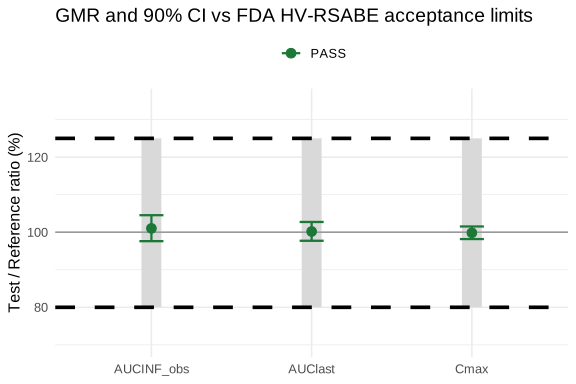
The grey band is each parameter's acceptance window (here everywhere 80-125% → nothing scaled); the dashed lines mark the fixed 80-125% reference and the solid line marks 100%.

References

Source: [1] (Howe, W. G. (1974). Approximate Confidence Limits on the Mean of X + Y Where X and Y Are Two Tabled Independent Random Variables. Journal of the American Statistical Association 69(347):789–794. Approximation I is the method FDA cites for obtaining the 95% upper confidence bound)

Last updated: September 28, 2026