How to back transform the VPC and individual fits
In some cases, a transformation is applied to both the observation and the prediction. One example would be transforming the observation in an MBMA analysis to weight the residual error or apply a logit transformation. The transformation is applied to both the observation in the dataset and the prediction in the structural model. This means that the various diagnostic plots, such as the VPC and individual fits, are on the transformed scale, rather than the more easily interpretable original scale.
R code
The following functions can be used to back transform the VPC and individual fits plots in order to plot the untransformed observations and predictions.
# back transform plots for which the observation was transformed and / or weighted by another column
# this script is intended to be used with version 2024 of MonolixSuite and lixoftConnectors

library(ggplot2)
library(dplyr)
library(lixoftConnectors)


#' Backtransform Individual Fits and VPC
#'
#' In the case that the observed data has been transformed or weighted, this function provides the data frames necessary
#' to plot the individual fits and VPC for the model on the backtransformed scale of the data, which is generally more interpretable.
#'
#' The back transformation follows three steps (all optional), which depend on which arguments are provided:
#' (1) transform \code{weightingCol} with the function \code{weightingFunc}, (2) divide outputs by the
#' \code{weightingCol}, and (3) trandform the outputs according to the specified \code{link} and/or \code{backTransFunction}.
#'
#' First the unweighting, if specified, is applied by dividing by the weighting column. The weighting column can optionally
#' have a function applied first in tha case the \code{weightingFunc} is specifed. For example, if the variance of the residual
#' error is weighted by N, the number of individuals (and thus the standard deviation by sqrt(N)),
#' then weightingFunc = "sqrt" could be used. The weighting column is generally tagged as a regressor. The same project setting,
#' lastCarriedForward or linearInterpolation, will be used to interpolate the value for the predictions for the individual fits.
#'
#' Then after the unweighting, the backtransformation, if any, is applied. Standard transformations (logit and log) are supported,
#' or a custom function can be specified instead or in addition. See the example, which uses a logit link, then multiplies by 100
#' to convert to a percentage.
#'
#' @param projectFile the .mlxtran Monolix project file
#' @param obsName the name of the observation (in dataset header)
#' @param weightingCol (optional) the name of the weighting column (tagged as a regressor in the dataset)
#' @param weightingFunc (optional) a function to apply to the values in the weightingCol (e.g., "sqrt")
#' @param link (optional) the link function used to transform the data (so the inverse will be used to backtransform),
#' supported values are "logit" and "log"
#' @param backTransFunction (optional) a function instead of or in addition to the link argument, which will be applied
#' after the link function if both are specified
#'
#' @return a list with two data frames: obs which contains the backtransformed observations, and either fit, in the case of
#' individual fits which contains the backtransformed predictions (individual fits), or sim, in the case of VPC which contains
#' the VPC simulations. These data frames are those for the charts data with the same columns,
#' plus additional columns with the suffix "_backTrans" for the backtransformed values.
#'
#' @examples
#' # the following is an example used the MBMA case study
#' # the Monolix project and supporting files can be downloaded from
#' # https://monolixsuite.slp-software.com/tutorials/2024R1/case-study-longitudinal-model-based-meta-analysis-
#'
#'
#' projFile = "r03_variability1stage_groupeddrug.mlxtran"
#'
#' # individual fits
#' indFits = backtransformIndividualFits(projFile, "transY", weightingCol = "Narm", weightingFunc = "sqrt",
#'                                       link = "logit", backTransFunction = function(x) x*100)
#' indFits$obs$STUDY_ARM = paste(indFits$obs$ID, indFits$obs$ARM, sep = "#")
#' indFits$fit$STUDY_ARM = paste(indFits$fit$ID, indFits$fit$ARM, sep = "#")
#'
#' ggplot(data = indFits$obs, aes(x = time, y = transY_backTrans)) +
#'   geom_point(col = "darkblue") +
#'   geom_line(data = indFits$fit, aes(x = time, y = indivPredMode_backTrans), col = "purple", lwd = 1) +
#'   facet_wrap(vars(STUDY_ARM), scales = "free") +
#'   ylab("ACR20") +
#'   theme_classic()
#'
#' # VPC (uses package vpc to create the plot)
#' vpcData = backtransformVpc(projFile, "transY", weightingCol = "Narm", weightingFunc = "sqrt",
#'                            link = "logit", backTransFunction = function(x) x*100)
#' vpc(sim = vpcData$sim, obs = vpcData$obs,
#'     obs_cols = list(dv = "transY_backTrans", idv = "time", id = "ID"),
#'     sim_cols = list(dv = "sim_transY_backTrans", idv = "time", id = "ID")) +
#'   ylab("ACR20")
#'
#' # vpc using the same bins as Monolix
#'
#' computeChartsData("vpc")
#' bin_data = read.csv("r03_variability1stage_groupeddrug/ChartsData/VisualPredictiveCheck/transY_bins.txt")
#'
#' vpc(sim = vpcData$sim, obs = vpcData$obs,
#'     obs_cols = list(dv = "transY_backTrans", idv = "time", id = "ID"),
#'     sim_cols = list(dv = "sim_transY_backTrans", idv = "time", id = "ID"),
#'     bins = bin_data$bins_values) +
#'   ylab("ACR20")+
#'   theme_classic()
#'
backtransformIndividualFits = function(projectFile, obsName,
                                       weightingCol = NULL, weightingFunc = NULL,
                                       link = NULL, backTransFunction = NULL)
{
  initializeLixoftConnectors("monolix", force = TRUE)
  loadProject(projectFile)

  if (!getLaunchedTasks()$conditionalModeEstimation) stop("Run the conditionalModeEstimation task first")

  projDir = dirname(projectFile)
  projName = tools::file_path_sans_ext(basename(projectFile))

  computeChartsData("indfits", output = obsName)

  chartDir = file.path(projDir, projName, "ChartsData/IndividualFits")
  indivFit = read.csv(file.path(chartDir, paste0(obsName, "_fits.txt")))
  indivObs = read.csv(file.path(chartDir, paste0(obsName, "_observations.txt")))

  # remove any duplicated rows which cause problems in join
  indivFit = indivFit[!duplicated(indivFit),]

  dataInfo = getDatasetInfo(weightingCol)

  interpMethod = switch(getData()$regressorsSettings,
                        "lastCarriedForward" = "constant",
                        "linearInterpolation" = "linear")

  # join dataset (obs time) with fit plot data (pred time),
  # so that we can interpolate the weight column at pred time
  chartCols = c("ID", dataInfo$occCol, "time")
  dataCols = c(dataInfo$idCol, dataInfo$occCol, dataInfo$timeCol)

  dataset_pred = dataInfo$dataset %>%
    full_join(select(indivFit, all_of(chartCols)),
              by = setNames(nm = dataCols, chartCols)) %>%
    arrange(across(all_of(dataCols)))

  # need to interpolate by id/occ
  dataset_pred$id_occ = apply(dataset_pred[,c(dataInfo$idCol, dataInfo$occCol)], 1, paste, collapse = " ")
  dataset_pred$id_occ = factor(dataset_pred$id_occ, levels = unique(dataset_pred$id_occ)) # keep order as in dataset
  dataset_pred[,weightingCol] = unlist(by(dataset_pred,
                                          dataset_pred$id_occ,
                                          function(df) approx(x = df[,dataInfo$timeCol],
                                                              y =df[,weightingCol],
                                                              xout = df[,dataInfo$timeCol],
                                                              method = interpMethod)$y))

  if (!is.null(weightingFunc))
  {
    weightingFunc = match.fun(weightingFunc)
    dataset = dataInfo$dataset %>%
      mutate(across(.cols = as.name(weightingCol),
                    .fns = ~ weightingFunc(.)))
    dataset_pred = dataset_pred %>%
      mutate(across(.cols = as.name(weightingCol),
                    .fns = ~ weightingFunc(.)))
  }

  ## transform observation data ##

  obsColsToTransform = c(obsName, "median", "piLower", "piUpper")

  indivObs = weightAndTransformDf(indivObs, dataset,
                                  dataInfo$idCol, dataInfo$occCol, dataInfo$timeCol, weightingCol,
                                  obsColsToTransform, link, backTransFunction)


  ## transform fit data ##

  fitColsToTransform = c("pop", "popPred", "indivPredMean", "indivPredMode")

  indivFit = weightAndTransformDf(indivFit, dataset_pred,
                                  dataInfo$idCol, dataInfo$occCol, dataInfo$timeCol, weightingCol,
                                  fitColsToTransform, link, backTransFunction)

  return(list(obs = indivObs, fit = indivFit))

}

#' See backtransformIndividualFits
#'
backtransformVpc = function(projectFile, obsName,
                            weightingCol = NULL, weightingFunc = NULL,
                            link = NULL, backTransFunction = NULL)
{
  initializeLixoftConnectors("monolix", force = TRUE)
  loadProject(projectFile)

  projDir = dirname(projectFile)
  projName = tools::file_path_sans_ext(basename(projectFile))

  computeChartsData(plot = "vpc", output = obsName, exportVPCSimulations = TRUE)

  chartDir = file.path(projDir, projName, "ChartsData/VisualPredictiveCheck")
  simData = read.csv(file.path(chartDir, paste0(obsName, "_simulations.txt")))
  obsData = read.csv(file.path(chartDir, paste0(obsName, "_observations.txt")))

  dataInfo = getDatasetInfo(weightingCol)

  if (!is.null(weightingFunc))
  {
    weightingFunc = match.fun(weightingFunc)
    dataset = dataInfo$dataset %>%
      mutate(across(.cols = as.name(weightingCol),
                    .fns = ~ weightingFunc(.)))
  }

  ## transform observation data ##

  obsColsToTransform = obsName

  # obs for VPC already has Narm, remove it since we add it from the interpreted data
  obsData = weightAndTransformDf(select(obsData, -all_of(weightingCol)), dataset,
                                 dataInfo$idCol, dataInfo$occCol, dataInfo$timeCol, weightingCol,
                                 obsColsToTransform, link, backTransFunction)


  ## transform simulations ##

  simColsToTransform = paste0("sim_", obsName)

  # note: don't need to interpolate as simulations are at observed time points
  simData = weightAndTransformDf(simData, dataset,
                                 dataInfo$idCol, dataInfo$occCol, dataInfo$timeCol, weightingCol,
                                 simColsToTransform, link, backTransFunction)

  return(list(obs = obsData, sim = simData))

}

getDatasetInfo = function(weightingCol)
{
  dataInfo = getData()
  if (sum(dataInfo$headerTypes == "occ") != 1) stop("Must have exactly 1 occasion column")
  occCol = dataInfo$header[dataInfo$headerTypes == "occ"]
  idCol = dataInfo$header[dataInfo$headerTypes == "id"]
  timeCol = dataInfo$header[dataInfo$headerTypes == "time"]

  # get dataset from project for weighting
  dataset = getInterpretedData()
  dataset = dataset %>%
    select(all_of(c(idCol, occCol, timeCol, weightingCol))) %>%
    mutate(across(all_of(c(occCol, timeCol, weightingCol)), as.numeric))

  # set ID (aka study) as numeric if it is, for later join
  origID = dataset[,idCol]
  tryCatch(expr = { dataset[,idCol] <- as.numeric(dataset[,idCol]) },
           warning = function(e){ dataset[,idCol] <- origID })

  return(list(dataset = dataset, idCol = idCol, timeCol = timeCol, occCol = occCol))
}


weightAndTransformDf = function(df, weights,
                                idCol, occCol, timeCol, weightingCol,
                                colsToTransform, link, backTransFunction)
{
  # create new columns
  df = df %>%
    mutate(across(.cols = all_of(colsToTransform),
                  .names = "{col}_backTrans"))
  colsTrans = paste0(colsToTransform, "_backTrans")

  # weighting
  if (!is.null(weightingCol))
  {
    df = df %>%
      left_join(weights, by = setNames(nm = c("ID", occCol, "time"), c(idCol, occCol, timeCol))) %>%
      mutate(across(.cols = all_of(colsTrans),
                    .fns = ~ ./ !!as.name(weightingCol))) %>% #!!as.name() !!sym()
      select(-any_of(weightingCol))
  }

  # backtransform
  if (!is.null(link))
  {
    if (link == "logit")
    {
      df = df %>%
        mutate(across(.cols = all_of(colsTrans),
                      .fns = ~ exp(.) / (1 + exp(.))) )
    } else if (link == "log")
    {
      df = df %>%
        mutate(across(.cols = all_of(colsTrans),
                      .fns = ~ exp(.)) )
    }
  }
  if (!is.null(backTransFunction))
  {
    backTransFunction = match.fun(backTransFunction)

    if (is.function(backTransFunction))
    {
      df = df %>%
        mutate(across(.cols = all_of(colsTrans),
                      .fns = ~ backTransFunction(.)))
    }
  }

  return(df)
}
Examples
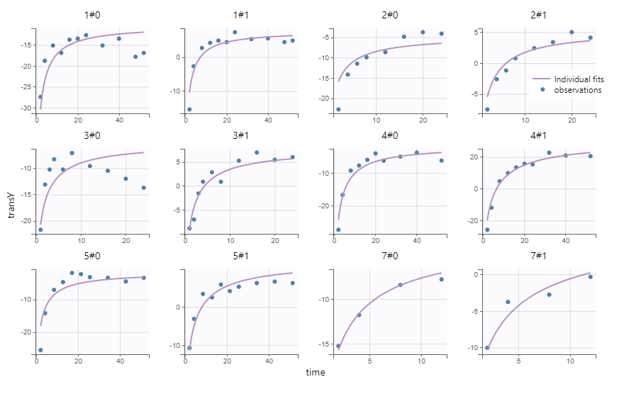
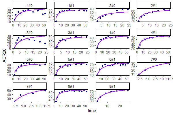
Individual fits
Here is an example of plotting the untransformed individual fits for the Monolix project from the MBMA analysis, where the project is available for download. The observation was weighted by the square root of Narm, the number of individuals per arm. Additionally, the response variable ACR20 is a percent, so there is a logit transformation as well as multiplication by 100 to shift from [0,1] to [0,100]. The function backtransformIndividualFits returns a list with two data frames, obs and fit, for the back transformed observations and predictions. These data frames can be used to create the individual fit plots.
projFile = "r03_variability1stage_groupeddrug.mlxtran"

# individual fits
indFits = backtransformIndividualFits(projFile, "transY",
                                      weightingCol = "Narm",
                                      weightingFunc = "sqrt",
                                      link = "logit",
                                      backTransFunction = function(x) x*100)
indFits$obs$STUDY_ARM = paste(indFits$obs$ID, indFits$obs$ARM, sep = "#")
indFits$fit$STUDY_ARM = paste(indFits$fit$ID, indFits$fit$ARM, sep = "#")

ggplot(data = indFits$obs, aes(x = time, y = transY_backTrans)) +
  geom_point(col = "darkblue") +
  geom_line(data = indFits$fit, aes(x = time, y = indivPredMode_backTrans),
            col = "purple", lwd = 1) +
  facet_wrap(vars(STUDY_ARM), scales = "free") +
  ylab("ACR20") +
  theme_classic()
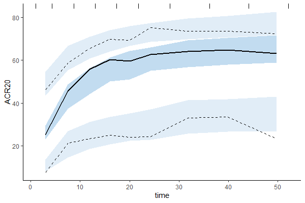
VPC
Next, with the same project, we can also plot the VPC. The function backtransformVpcreturns a list with two data frames, obs and sim, for the back transformed observations and simulations. This uses the R package vpc to create the VPC plot, which could also be created manually or with a different package based on the back transformed VPC simulations.
projFile = "r03_variability1stage_groupeddrug.mlxtran"
library(vpc)

# VPC (uses package vpc to create the plot)
vpcData = backtransformVpc(projFile, "transY",
                           weightingCol = "Narm",
                           weightingFunc = "sqrt",
                           link = "logit",
                           backTransFunction = function(x) x*100)
vpc(sim = vpcData$sim, obs = vpcData$obs,
    obs_cols = list(dv = "transY_backTrans", idv = "time", id = "ID"),
    sim_cols = list(dv = "sim_transY_backTrans", idv = "time", id = "ID")) +
  ylab("ACR20")