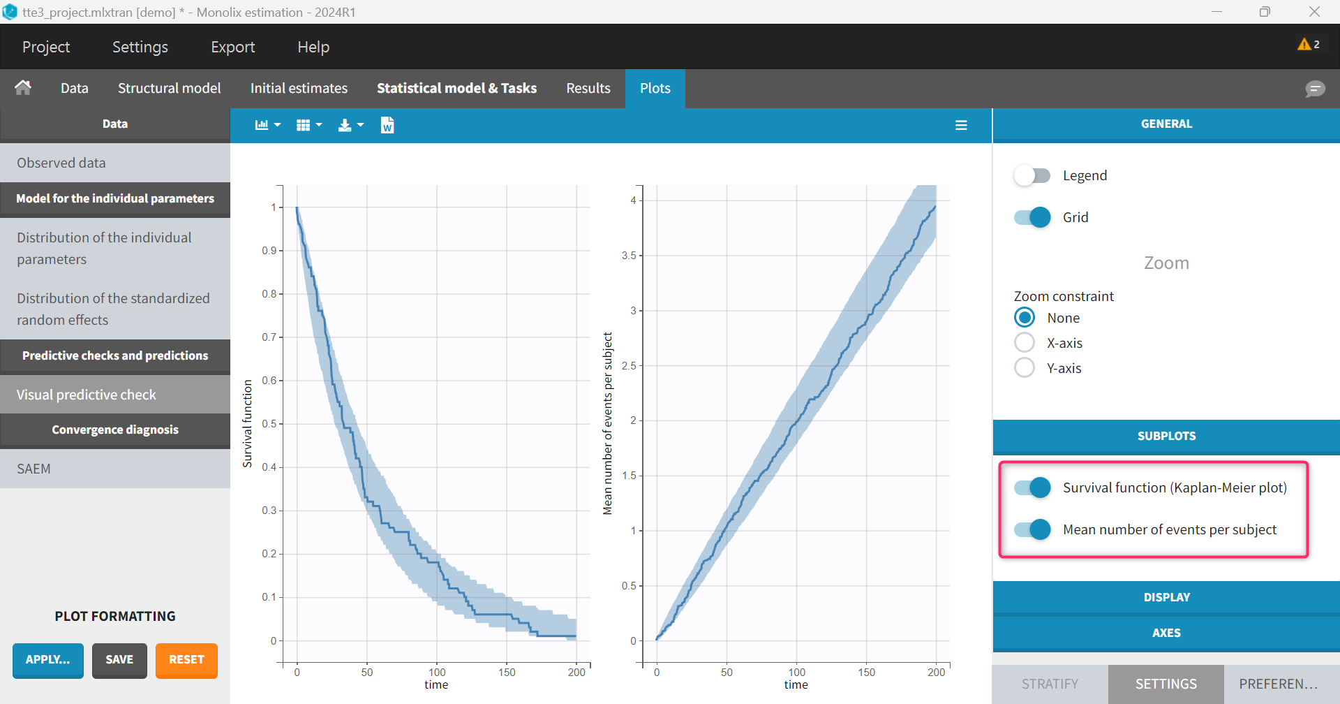
VPCs for every event for repeated time-to-event data

In case of repeated time-to-event data, Monolix VPC plot shows the Kaplan-Meier (KM) for the first event, as well as the mean number of events per subject (cumulative plot).

It is not possible to display in the GUI the KM plot for the second or third event for instance. However, this can be done in R.

The general workflow is the following:

use the lixoftConnectors to load the project and export the VPC simulations using computeChartsData(plot="vpc", exportVPCSimulations = T) [this step can be skipped if the VPC simulations are exported via the GUI using Export > Export VPC simulations]
read the original data as well as the simulated data
filter the original and simulate data to keep only the nth event
use survfit from the survival package to generate a KM curve for the original data and each replicate of the simulated data. A time grid must be specified in order to get the KM curve on the same times for all replicates.
calculate percentiles over replicates for the simulated data
plot the oroginal KM curve and prediction interval using ggplot2

An example is shown below using the tte3_project.mlxtran from the demos.

R

library(lixoftConnectors)
initializeLixoftConnectors(software="monolix")
library(survival)
library(dplyr)
library(ggplot2)

# project from teh demos
proj <- paste0(getDemoPath(),"/3.models_for_noncontinuous_outcomes/3.3.time_to_event_data_model/tte3_project.mlxtran")

# load project using lixoftConnectors
loadProject(proj)

# export VPC simulations (can also be done via the GUI)
computeChartsData(plot="vpc", exportVPCSimulations = T)

# read file containing simulated data
sim_data <- read.csv(paste0(tools::file_path_sans_ext(proj),"/ChartsData/VisualPredictiveCheck/Event_simulations.txt"))

# read file containing original data (dataset)
obs_data <- read.csv(getData()$dataFile, sep=" ")

# max number of events to display
nmax <- 4

# containers
predInterv_allEvents <- NULL
KMoriginal_allEvents <- NULL

# for each nth events
for(i in 1:nmax){
  print(paste0("Event number ",i))
  
  # for each id and rep, filter to keep first row (DV=0), nth event (row n+1) and last row (DV=0)
  sim_nth <- sim_data %>% group_by(rep,ID) %>% filter(row_number()==1 | row_number()==(i+1) | row_number()==n()) %>% ungroup()
  obs_nth <- obs_data %>% group_by(ID)     %>% filter(row_number()==1 | row_number()==(i+1) | row_number()==n()) %>% ungroup()
  
  # create KM curve for each replicate (can be extended to do each replicate and each stratification group)
  # it is important to add the "times" argument to get all KM curves on the same time grid (in order to calculate percentiles later)
  KMcurves <- summary(survfit(Surv(time, sim_Event) ~ rep, data = sim_nth), times = seq(0,200,by=2))
  
  # survfit summary object to data.frame object
  KMcurves_df <- do.call(data.frame, lapply(c("time","surv","strata") , function(x) KMcurves[x]))
  
  # calculate percentiles for each time point 
  predInter <- KMcurves_df %>% group_by(time) %>% summarise(p05 = quantile(surv,0.05),
                                                            p95 = quantile(surv,0.95)) %>% ungroup() %>% mutate(EventNumber=paste0(i,"th event"))
  
  # create KM curve for original data
  KMcurveOriginal    <- summary(survfit(Surv(TIME, Y) ~ 1, data = obs_nth), times = seq(0,200,by=2))
  KMcurveOriginal_df <- do.call(data.frame, lapply(c("time","surv") , function(x) KMcurveOriginal[x])) %>% mutate(EventNumber=paste0(i,"th event"))
  
  # bind together
  predInterv_allEvents <- rbind(predInterv_allEvents,predInter)
  KMoriginal_allEvents <- rbind(KMoriginal_allEvents,KMcurveOriginal_df)
  
}

# EventNumber as factor
KMoriginal_allEvents$EventNumber <- as.factor(KMoriginal_allEvents$EventNumber)
predInterv_allEvents$EventNumber <- as.factor(predInterv_allEvents$EventNumber)

# plot prediction interval with overlay of actual KM curve, stratified by EventNumber
ggplot()+geom_line(data=KMoriginal_allEvents, aes(x=time,y=surv), size=0.5)+
  geom_ribbon(data=predInterv_allEvents, aes(x=time, ymin=p05, ymax=p95), alpha=0.5, fill="#00a4c6") +
  facet_wrap(~EventNumber) + theme_bw()+
  ylab("Survival") + xlab("Time")

We obtain the following plot: