Package "mlxModelFinder"

Introduction and Advantages

Model selection is at the heart of pharmacometric analysis. Deciding between one- vs two-compartment models, choosing the right absorption mechanism, or testing for lag time can easily result in dozens of candidate models. Manually exploring all of these is tedious and error-prone.

The findModel() function automates this exploration. Instead of manually editing model files, you can define the search space explicitly and let the function:

• Explore efficiently: Test large numbers of candidate models with minimal manual work.

• Ensure reproducibility: Fix seeds and record the search process.

• Adapt to your needs: Choose among different algorithms optimized for small or large search spaces.

• Provide transparency: Return a structured table of results with clear metrics and convergence information.

This approach frees you from repetitive tasks and allows you to focus on interpreting results and making scientific decisions.

Download and Installation

You can download the package from mlxModelFinder_2.0.1.tar.gz.

Requirements

The package has the following dependencies:

Imports (required):

• lixoftConnectors

• cli

Suggests (optional):

• htmltools and plotly for plotting algorithm convergence in real time

• testthat, withr

• data.tree and DiagrammeR for plotting the decision tree diagram

• xgboost for optimizing ACO

• future and future.apply for parallel execution

Installation Example

install.packages("mlxModelFinder_2.0.0.tar.gz", repos = NULL, type = "source")

Algorithms Used

The package implements and benchmarks several algorithms. Each algorithm has different strengths, so you can pick the one that best suits your problem or let the function pick the most suitable algorithm:

• Decision Tree (DT)
  A fast, greedy algorithm that works well when inter-individual variability (IIV) is not part of the search. It quickly narrows down to a strong candidate structure. Only supports the built-in PK library (library = "pk").

• Ant Colony Optimization (ACO)
  A stochastic, population-based algorithm where many “ants” explore the model space and share information. Particularly effective when exploring complex spaces that include IIV. Supports parallel execution.

• Exhaustive Search
  Tests all possible models in the search space. Useful when the space is small enough to allow it, and when you want a complete overview. Supports parallel execution.

Function Reference

Usage

findModel(
  project,
  library,
  requiredFilters,
  filters = NULL,
  algorithm = NULL,
  settings = NULL,
  metric_func = NULL,
  initial_func = NULL,
  model_creation_func = NULL,
  param_mapping = NULL,
  param_distributions = NULL,
  fixed_iiv = NULL,
  obs_mapping = NULL
)

Arguments

Examples

Here are examples illustrating how each algorithm can be used.

Decision Tree

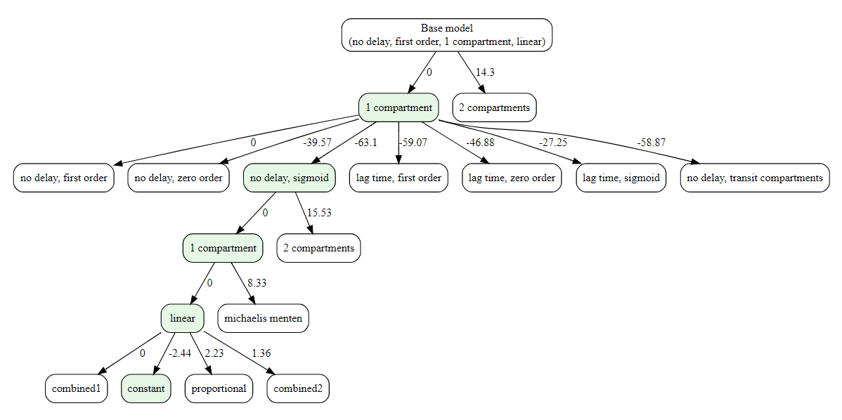
The decision-tree search starts from the simplest model and iteratively grows it: at each step, it replaces one structural component (e.g., absorption, delay, distribution, elimination) with a more complex alternative only if the metric improves. This greedy process continues until no single change yields a better score. If settings$plot is TRUE (default), a diagram of the explored path is produced.

library(lixoftConnectors)
initializeLixoftConnectors()

results <- findModel(
    project = file.path(getDemoPath(), "1.creating_and_using_models",
                        "1.1.libraries_of_models", "theophylline_project.mlxtran"),
    library = "pk",
    algorithm = "decision_tree",
    requiredFilters = list(administration = "oral", parametrization = "clearance"),
    settings = list(findIIV = FALSE, findError = TRUE)
)

#> ℹ Search space size: 252 models
#> 
#> ── Initializing Decision Tree Search ──────────────────────
#> 
#> ── Optimizing distribution 
#> ✔ Done. Selected: 1compartment
#> 
#> ── Optimizing absorption_delay 
#> ✔ Done. Selected: noDelay, sigmoid
#> 
#> ── Optimizing distribution 
#> ✔ Done. Selected: 1compartment
#> 
#> ── Optimizing elimination 
#> ✔ Done. Selected: linear
#> 
#> ── Optimizing error model 
#> ✔ Done

Ant Colony Optimization

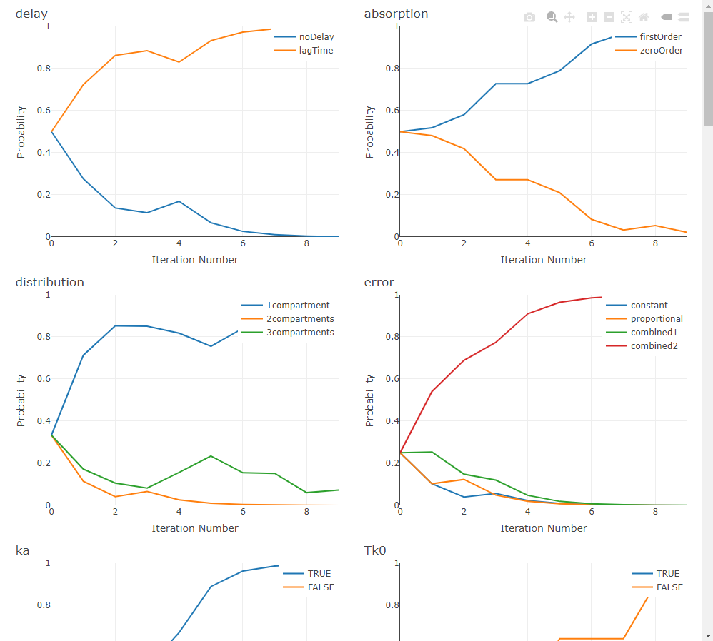
ACO treats model selection as a guided search through the space of structural choices. A population of “ants” samples complete models by following a probability matrix over components (e.g., absorption, delay, distribution, elimination). After each iteration, probabilities are reinforced toward the better-scoring models (pheromone update) and evaporate elsewhere (controlled by rho), striking a balance between exploitation of good patterns and exploration of new ones. The process repeats until the stopping rule is met.

In practice, ACO shines when the search space is large—especially when you also explore IIV and residual-error structures—because it learns which structural choices tend to co-occur in high-performing models, rather than testing combinations blindly.

When settings$plot is TRUE (and the optional plotly/htmltools are available), ACO renders live progress plots—tracking per-component selection probabilities (pheromones), the best metric by iteration, and convergence status—so you can visually monitor how the swarm is learning.

results <- findModel(
  project = file.path(getDemoPath(), "6.PK_models", "6.2.multiple_routes",
                      "ivOral1_project.mlxtran"),
  library = "pk",
  algorithm = "ACO",
  requiredFilters = list(administration = "oralBolus", parametrization = "rate"),
  filters = list(absorption = c("zeroOrder", "firstOrder"),
                 elimination = "linear"),
  settings = list(findIIV = TRUE, findError = TRUE)
)

#> ℹ Search space size: 24192 models
#> 
#> ── Initializing ACO Search ───────────────────────────
#> 
#> ── Iteration 1 ──
#> 
#> Running models ■■■■■■■■■■■■■■■■■■■■■■■■■■■■■■■  | 20/20
#> ℹ Total number of models tested so far: 17
#> ℹ Best model found so far:
#> • delay: noDelay
#> • absorption: zeroOrder
#> • distribution: 1compartment
#> • elimination: linear
#> • bioavailability: true
#> • IIV Tk0: TRUE
#> • IIV V: TRUE
#> • IIV k: TRUE
#> • IIV F: TRUE
#> • error: proportional
#> • metric: 1230.5
#> 
#> ── Iteration 2 ──
#> 
#> Running models ■■■■■■■■■■■■■■■               | 10/20
#> ...

Exhaustive Search

It will test all of the models.

results <- findModel(
    project = file.path(getDemoPath(), "1.creating_and_using_models",
                        "1.1.libraries_of_models", "theophylline_project.mlxtran"),
    library = "pk",
    algorithm = "exhaustive_search",
    requiredFilters = list(administration = "oral", parametrization = "clearance"),
    settings = list(findIIV = FALSE, findError = TRUE)
)

#> ℹ Search space size: 252 models
#> Running models ■■■■■■■■■■■■■■■■■■■■■■■■■■■■■■■  | 100%
#> ✔ Done

Custom Model Library

Custom models let you search over any model structures -- not just the built-in PK library. You provide a model_creation_func that maps filter combinations to models. See the "Going Beyond the Built-in Model Libraries" page for detailed examples, including:

• Using the Monolix PKPD library with getLibraryModelName() to search over PD structures with a fixed PK model

• Building model files programmatically for non-standard PK features (saturable absorption, dose-dependent bioavailability)

• Optimizing IIV configurations on a single complex model

# Example: search over PD turnover models with fixed PK
model_func <- function(library, filters) {
  fixed_filters <- list(
    administration = "oral", delay = "lagTime",
    absorption = "firstOrder", distribution = "1compartment",
    elimination = "linear", parametrization = "clearance"
  )
  all_filters <- c(fixed_filters, filters)
  lixoftConnectors::getLibraryModelName("pkpd", all_filters)
}

result <- findModel(
  project = "my_pkpd_project.mlxtran",
  library = "custom",
  filters = list(
    response = "turnover",
    drugAction = c("productionStimulation", "productionInhibition",
                   "degradationStimulation", "degradationInhibition")
  ),
  model_creation_func = model_func,
  param_mapping = list(
    common_params = c("Tlag", "ka", "V", "Cl", "R0", "kout"),
    filter_params = list(
      drugAction = list(
        productionStimulation  = c("Emax", "EC50"),
        productionInhibition   = c("Imax", "IC50"),
        degradationStimulation = c("Emax", "EC50"),
        degradationInhibition  = c("Imax", "IC50")
      )
    )
  ),
  algorithm = "ACO",
  settings = list(findIIV = TRUE, findError = TRUE)
)

Providing Custom Metric Function

By default, findModel() uses BICc as the scoring metric. When the search includes inter-individual variability (IIV), the default is BICc plus a penalty for unstable parameter estimates: every RSE above 50% contributes a penalty proportional to the number of observations.
We chose this default after thorough benchmarking across simulated and real datasets, where it showed the best balance between accuracy and robustness.

Still, you may prefer a different metric—for example, AIC—depending on your project or organizational standards. For that, you can provide your own metric function.

Example: AIC metric

findModel() expects a zero-argument function. After each Monolix run, your function is called and should return a single numeric score (lower is better). You retrieve results via lixoftConnectors.

my_aic_metric <- function() {
  # Choose the likelihood source consistently with your workflow:
  # - "linearization" pairs with linearized likelihoods
  # - otherwise use "importanceSampling" for final scoring
  method <- if (exists("settings", inherits = TRUE) && isTRUE(get("settings")$linearization)) {
    "linearization"
  } else {
    "importanceSampling"
  }

  ll_info <- lixoftConnectors::getEstimatedLogLikelihood()[[method]]

  # Try to read AIC by name; if names are unavailable, fall back to the first element.
  aic <- tryCatch({
    if (!is.null(names(ll_info)) && "AIC" %in% names(ll_info)) {
      as.numeric(ll_info[["AIC"]])
    } else {
      as.numeric(ll_info[[1L]])
    }
  }, error = function(e) NA_real_)

  # Be defensive: if AIC is missing, return a very large penalty so this model ranks poorly.
  if (is.na(aic)) return(1e12)

  return(aic)
}

Notes and good practices

• Zero arguments only. Your function cannot take parameters; read everything you need via lixoftConnectors.

• Lower is better. If you ever want to maximize a quantity, just return its negative value.

• Be defensive. When values are missing (e.g., non-convergence), return a large number (e.g., 1e12) so such runs sort to the bottom.

• Stay consistent with estimation. If you evaluate AIC from linearization, keep it consistent with how the run’s likelihood was computed (the example switches to "linearization" when appropriate).

• Custom tasks. If your metric function requires specific Monolix tasks (e.g., importance sampling for log-likelihood), make sure they are enabled in settings$tasks.

Using it in findModel()

res <- findModel(
  project = "theophylline_project.mlxtran",
  library = "pk",
  requiredFilters = list(administration = "oral", parametrization = "clearance"),
  # optional: filters / algorithm / settings ...
  metric_func = my_aic_metric
)

If you prefer to penalize unstable models, you can build on top of AIC the same way the default metric does with RSEs. For example, after computing aic, add a term like
aic + (# high RSEs) * log(n_obs) by retrieving standard errors via getEstimatedStandardErrors() and the observation count via getObservationInformation().

Providing custom initial estimates

findModel() accepts an initial_func that must take one argument—the project path—and must return a project path (either the same path, or a new one). Inside this function you should:

1. Load the project with lixoftConnectors.

2. Read the population-parameter table.

3. Apply your initial values.

4. Save the project (same file or a new file) and return the path you saved.

Name mapping tip: Population fixed effects are typically named like ka_pop, V_pop, etc. If you provide initials keyed by individual parameter names (e.g., ka, V), map them to paste0(name, \"_pop\"). If you already use the exact names in the population table, no mapping is needed.

Example — Apply a predefined list of initials

This example takes a user-supplied list (e.g., list(ka = 1.2, V = 25, k = 0.12, Cl = 3.0)) and writes those values into the project’s population parameter table. The example uses the function applyInitials that comes with the package and allows to easily provide initial values. Unmatched names are ignored safely. The parameter values not defined in my_inits will be set to Monolix defaults.

# Predefined initials (mix of individual names and/or population-table names)
my_inits <- list(
  ka = 1.2,   # maps to ka_pop if present
  V  = 25,    # maps to V_pop
  k  = 0.12,  # maps to k_pop
  Cl = 3.0,   # if population table has "Cl_pop", set that via mapping from "Cl"
  Q  = 1.5,   # maps to Q_pop
  V2 = 15     # maps to V2_pop
)

res <- findModel(
  project = "theophylline_project.mlxtran",
  library = "pk",
  requiredFilters = list(administration = "oral", parametrization = "clearance"),
  filters = list(distribution = c("1compartment", "2compartments"),
                 absorption = "firstOrder",
                 elimination = "linear"),
  initial_func = applyInitials(my_inits)
)

Appending Custom Columns to Results

By default, findModel() returns a results table containing the structural model filters, IIV configuration, error model, and the metric score. Sometimes you want additional diagnostics for each run -- for example, OFV alongside BICc, the number of poorly estimated parameters, or any other quantity available after a Monolix run.

The settings$table_func setting lets you do exactly that. You provide a zero-argument function that is called after each model run, when lixoftConnectors still holds the results of the most recent estimation. The function must return a single-row data.frame whose columns are appended to that model's result row.

This is particularly useful for:

• Comparing multiple information criteria (AIC, BIC, BICc) side by side without re-running models

• Recording diagnostic flags such as the number of parameters with high RSE, shrinkage values, or condition numbers

• Capturing run metadata like estimated parameter values or convergence status

my_table_func <- function() {
  se <- lixoftConnectors::getEstimatedStandardErrors()$stochasticApproximation

  # Count how many parameters have RSE > 50%
  n_high_rse <- sum(se$rse > 50, na.rm = TRUE)

  # Get the log-likelihood values
  ll <- lixoftConnectors::getEstimatedLogLikelihood()$importanceSampling

  list(
    AIC = ll[["AIC"]],
    BIC = ll[["BIC"]],
    n_high_rse = n_high_rse
  )
}

result <- findModel(
  project = "my_project.mlxtran",
  library = "pk",
  requiredFilters = list(administration = "oral", parametrization = "clearance"),
  settings = list(
    iiv = TRUE,
    error = TRUE,
    table_func = my_table_func
  )
)

print(result$results)
#>   absorption delay distribution elimination ka  V  Cl error    metric  AIC  BIC n_high_rse
#> 1 firstOrder noDelay 1compartment    linear TRUE TRUE TRUE combined  285.3 290.1 295.4          0
#> 2 firstOrder lagTime 1compartment    linear TRUE TRUE TRUE combined  287.1 292.5 298.0          1
#> ...