Dose proportionality assessment | MonolixSuite Documentation

Dose proportionality can be described when the systemic exposure (e.g. Cmax, AUC) increases in direct proportion to the administered dose amount, meaning doubling the dose doubles the exposure. Characterising how exposure changes with dose is a routine part of early pharmacokinetic analysis. When exposure is dose proportional, concentrations at an untested dose could be approximated by simple proportional scaling; departures from proportionality (supra- or sub-proportional increases) point to non-linear pharmacokinetics that require closer attention. The power-model assessment described here is a common exploratory tool for this purpose [Smith et al. 2000; Hummel et al. 2008].

Concept and mathematics

The assessment implemented here uses the power model, which relates a PK parameter to dose through

The model is fit via a linear regression of on ; the slope is the estimate of interest:

exact dose proportionality (exposure scales 1:1 with dose),
exposure increases more than proportionally
exposure increases less than proportionally

Because a point estimate of exactly is never observed, dose proportionality is assessed with an equivalence criterion (Smith et al. 2000; Hummel et al. 2008). Given the ratio of the highest to the lowest dose

and acceptance bounds for the ratio of dose-normalised exposures over that dose range, proportionality is concluded when the 90% confidence interval of lies entirely within that critical region

Choice of acceptance bounds

The bounds are set on the ratio of dose-normalised exposure between the extremes of the dose range, not on the slope directly. Two conventions are used in the literature:

Bounds	Origin	When appropriate
(0.80, 1.25)	Confidence Interval Criteria for Assessment of Dose Proportionality (Smith et al. 2000)	Strict; reasonable when doses are only ~2-fold apart. Becomes very hard to satisfy over a wide dose range.
(0.50, 2.00)	Exploratory assessment of dose proportionality: review of current approaches and proposal for a practical criterion (Hummel et al. 2008)	Allows a -fold change in dose-normalised exposure; intended for exploratory assessment over a wide dose range.

Both are symmetric on the log scale ( ). The bounds should be pre-specified in the analysis plan and justified by what fold-change in exposure is clinically acceptable.

Interpretation

The conclusion follows from the position of the 90% CI of the slope relative to the critical region where and

Position of the 90% CI of	Conclusion
Entirely inside	Proportional
Entirely outside (below or above)	Not proportional
Overlapping the interval	Inconclusive

Function `doseProportionality()`

The above explaned methodology can be implemented as follows: it requires the individual NCA parameters retrieved by getNCAIndividualParameters()$parameters and returns the assessment:

doseProportionality <- function(ds,                    # data set (longitudinal format)
                                parNm,                 # parameter name (label in the output table)
                                parVal  = "Value",     # column holding the parameter values
                                doseVal = "Dose",      # column holding the dose values
                                thetaL  = 0.5,         # lower acceptance bound for the dose-normalised ratio
                                thetaH  = 2.0)         # upper acceptance bound for the dose-normalised ratio
{
  # Keep only rows usable on the log-log scale (positive, finite dose and value).
  ok <- is.finite(ds[[doseVal]]) & is.finite(ds[[parVal]]) &
        ds[[doseVal]] > 0 & ds[[parVal]] > 0
  if (any(!ok))
    warning(sprintf("doseProportionality: dropping %d row(s) with non-positive/non-finite values.", sum(!ok)))
  ds <- ds[ok, , drop = FALSE]

  if (length(unique(ds[[doseVal]])) < 2)
    stop("doseProportionality: need at least two distinct dose levels.")

  # Clean two-column frame so the fitted models carry tidy variable names.
  fit_df   <- data.frame(param = ds[[parVal]], dose = ds[[doseVal]])

  rr       <- max(fit_df$dose) / min(fit_df$dose)       # highest / lowest dose
  parfit   <- lm(log(param) ~ log(dose), data = fit_df) # power fit
  beta.est <- unname(coef(parfit)[2])                   # slope estimate
  beta.int <- confint(parfit, level = 0.9)[2, ]         # 90% CI of the slope
  llim     <- 1 + log(thetaL) / log(rr)                 # critical region, lower limit
  ulim     <- 1 + log(thetaH) / log(rr)                 # critical region, upper limit

  # CI inside -> Proportional; straddling -> Inconclusive; outside -> Not Proportional.
  if (beta.int[1] > llim & beta.int[2] < ulim) {
    test.res <- "Proportional"
  } else if ((beta.int[1] <= llim & (beta.int[2] > llim & beta.int[2] < ulim)) |
             ((beta.int[1] > llim & beta.int[1] < ulim) & beta.int[2] >= ulim) |
             ( beta.int[1] <= llim & beta.int[2] >= ulim)) {
    test.res <- "Inconclusive"
  } else {
    test.res <- "Not proportional"
  }

  result.tab <- data.frame(parameter             = parNm,
                           `Dosing range`        = paste0(min(ds[[doseVal]]), "--", max(ds[[doseVal]])),
                           `Point estimate`      = round(beta.est, 2),
                           `Criteria interval`   = paste0("(", round(llim, 3), "; ", round(ulim, 3), ")"),
                           `Confidence interval` = paste0("(", round(beta.int[1], 3), "; ", round(beta.int[2], 3), ")"),
                           Conclusion            = test.res,
                           check.names           = FALSE)

  parfitlin <- lm(param ~ dose - 1, data = fit_df)       # through-origin fit, for plotting

  # Return the tidy table; attach data, models and numeric stats as attributes.
  attr(result.tab, "data")   <- fit_df
  attr(result.tab, "modlog") <- parfit
  attr(result.tab, "modlin") <- parfitlin
  attr(result.tab, "stats")  <- data.frame(beta = beta.est, ci_low = unname(beta.int[1]),
                                           ci_high = unname(beta.int[2]), llim = llim, ulim = ulim)
  result.tab
}

The core of the function is lm(log(param) ~ log(dose)): R's lm() fits a linear regression by ordinary least squares on the log-transformed data, so the fitted line is the power model on the log–log scale and its slope is the exponent . confint() then reads the 90% confidence interval of that slope off the fitted model. (The second fit, lm(param ~ dose - 1), is a plain through-origin line used only for plotting.)

Input data format

The function requires long-format data with one row per subject, containing (at least) a dose column and a parameter-value column. Only these two columns are used; extra columns are ignored.

id	Dose	parameter	Value
1	150	Cmax	12.3
2	150	Cmax	10.8
…	…	…	…

Point the function doseProportionality() at the relevant columns via parVal/doseVal (defaults "Value"/"Dose"), and set the acceptance bounds thetaL/thetaH . Call it once per parameter.

Example

Using the aPCSK9_SAD.pkx PKanalix demo project, we assess dose proportionality for Cmax, AUClast and AUCINF_obs.

Use the raw exposure parameters, not dose-normalised (_D). Pass the original Cmax / AUC parameters to doseProportionality(), not dose-normalised (_D) parameters. Dose-normalisation is already built in: under the dose-normalised exposure ratio is , so the bounds on map exactly onto the critical region for . A
_D parameter would give a slope of (proportionality at 0, not 1) and normalise the data twice, invalidating the criterion.

Via the lixoftConnectors we load the project with loadProject(), restrict the computed parameters to Dose, Cmax, AUClast and AUCINF_obs with setNCASettings(), run the analysis with runNCAEstimation(), and retrieve the individual NCA parameters with getNCAIndividualParameters()$parameters.

library(dplyr)
library(ggplot2)
path.software <- "C:/Program Files/Lixoft/MonolixSuite2024R1"
library(lixoftConnectors)
initializeLixoftConnectors(path.software, software = "pkanalix")
library(flextable)
##############################################################################
# helper to prepare the data
prepDataset <- function(ds,input_param){
  param <- sym(input_param)
  dt <- ds %>%
    dplyr::rename(Value=!!param)%>%
    mutate(parameter=input_param,
           Value    =as.numeric(Value))%>%
    select(id,Dose,parameter,Value)
  return(dt)
}
prj <- paste0(getDemoPath(),"/2.case_studies/project_aPCSK9_SAD.pkx")
loadProject(prj)

setNCASettings(computedNCAParameters=c("Dose","Cmax","AUClast", "AUCINF_obs"))
runNCAEstimation()

df_nca <- getNCAIndividualParameters()$parameters

df_nca <- rbind(prepDataset(df_nca, "Cmax"),
                prepDataset(df_nca, "AUClast"),
                prepDataset(df_nca, "AUCINF_obs"))

The retrieved table is in wide format (one column per parameter), so prepDataset() reshapes it into long format: one row per subject (id) and parameter, each row carrying the corresponding Dose. Once the dataset is in this format, doseProportionality() can be applied (once per parameter).

##############################################################################
# Dose proportionality analysis
# Assess each parameter; theta bounds set to the (0.5, 2.0) criterion
DP_params <- unique(df_nca$parameter)

tb.res   <- data.frame()
ci.res   <- data.frame()
stat.res <- data.frame()

for (i in DP_params) {
  nca.i <- df_nca %>% filter(parameter == i)
  res.i <- doseProportionality(ds     = nca.i, 
                               parNm  = i,
                              parVal  = "Value", 
                              doseVal = "Dose",
                              thetaL  = 0.5, 
                              thetaH  = 2.0)

  tb.res <- rbind(tb.res, res.i)

  # slope + 90% CI + critical region 
  st.i <- attr(res.i, "stats"); st.i$parameter <- i
  stat.res <- rbind(stat.res, st.i)

  # fitted line + 90% confidence / prediction bands (for the log-log plot)
  mdl.i  <- attr(res.i, "modlog")
  grid.i <- data.frame(dose = 10^seq(log10(min(nca.i$Dose)),
                                     log10(max(nca.i$Dose)), length.out = 100))
  ci.i   <- exp(predict(mdl.i, newdata = grid.i, interval = "confidence", level = 0.90))
  pi.i   <- exp(predict(mdl.i, newdata = grid.i, interval = "prediction", level = 0.90))
  ci.res <- rbind(ci.res,
                  data.frame(parameter = i, Dose = grid.i$dose,
                             fit = ci.i[, "fit"],
                             ci_lwr = ci.i[, "lwr"], ci_upr = ci.i[, "upr"],
                             pi_lwr = pi.i[, "lwr"], pi_upr = pi.i[, "upr"]))
}
flextable(tb.res) %>% autofit()

Interpretation: Over the 150–800 mg dose range, Cmax is dose‑proportional (β = 1.15; 90% CI 0.974–1.318, entirely within the acceptance region 0.586–1.414). For AUClast and AUCINF_obs the assessment is inconclusive (β = 1.27; 90% CI 1.067–1.474 and 1.074–1.474), since the upper CI bounds slightly exceeded the upper limit (1.414), which can indicate a possible tendency toward more‑than‑proportional total exposure.

Exposure vs. dose (log–log)

The power-model fit (solid), its 90% confidence interval (dashed) and 90% prediction interval (dotted) for each parameter:

ggplot(df_nca, aes(Dose, Value)) +
  geom_point(alpha = 0.6) +
  geom_line(data = ci.res, aes(Dose, fit,    linetype = "Power-model fit"),         colour = "#CD2626", linewidth = 1.2) +
  geom_line(data = ci.res, aes(Dose, ci_lwr, linetype = "90% confidence interval"), colour = "#1874CD", linewidth = 1.1) +
  geom_line(data = ci.res, aes(Dose, ci_upr, linetype = "90% confidence interval"), colour = "#1874CD", linewidth = 1.1) +
  geom_line(data = ci.res, aes(Dose, pi_lwr, linetype = "90% prediction interval"), colour = "#008B45", linewidth = 1.0) +
  geom_line(data = ci.res, aes(Dose, pi_upr, linetype = "90% prediction interval"), colour = "#008B45", linewidth = 1.0) +
  scale_linetype_manual(name   = NULL,
                        breaks = c("Power-model fit", "90% confidence interval", "90% prediction interval"),
                        values = c("Power-model fit"          = "solid",
                                   "90% confidence interval"  = "dashed",
                                   "90% prediction interval"  = "dotted")) +
  guides(linetype = guide_legend()) +  # green legend keys
  scale_x_log10() +
  scale_y_log10() +
  annotation_logticks(sides = "bl") +   
  facet_wrap(~ parameter, scales = "free_y") +
  labs(x = "log(Dose)", y = "log(Parameter value)") +
  theme_bw()

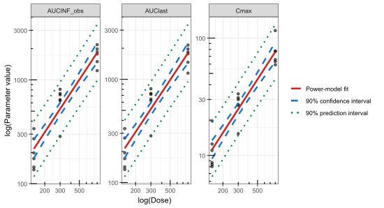
On the log–log scale, Cmax, AUClast and AUCINF_obs increased approximately linearly with dose (power‑model slopes near 1, all points within the 90% prediction interval).

Slope vs. critical region (decision plot)

The slope estimate (point estimate) and its 90% CI (bar) for each parameter, shown
vs the critical-region limits (dotted lines). A parameter is proportional when its CI lies entirely between the two limits. The limits are drawn as single vertical lines because all parameters share the same dose range. The critical region is identical for each parameter.

llim_val <- stat.res$llim[1]
ulim_val <- stat.res$ulim[1]

ggplot(stat.res, aes(x = beta, y = factor(parameter, levels = DP_params))) +
  geom_vline(xintercept = c(llim_val, ulim_val), linetype = "dotted", linewidth = 0.6) +
  geom_errorbarh(aes(xmin = ci_low, xmax = ci_high), height = 0.15) +
  geom_point(size = 2.5) +
  annotate("text", x = llim_val, y = Inf, label = "Lower limit", vjust = 1.4, fontface = "bold", size = 3.2) +
  annotate("text", x = ulim_val, y = Inf, label = "Upper limit", vjust = 1.4, fontface = "bold", size = 3.2) +
  scale_x_continuous(limits = c(0, max(2, max(stat.res$ci_high, ulim_val) * 1.05))) +
  coord_cartesian(clip = "off") +
  labs(title = "Dose proportionality evaluation",
       x = expression(beta ~ "with 90% CI"), y = NULL) +
  theme_bw() +
  theme(panel.grid  = element_blank(),
        plot.title  = element_text(hjust = 0.5, face = "bold"),
        plot.margin = margin(t = 18, r = 12, b = 6, l = 6))

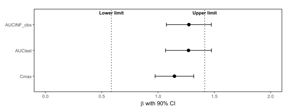
The power‑model slope with its 90% CI relative to the acceptance limits (0.586–1.414) shows Cmax lying fully within the region (dose‑proportional), whereas AUClast and AUCINF_obs intervals exceed the upper limit (inconclusive).

Last updated: July 15, 2026