Specific applications

This page covers analyses and use cases that go beyond the typical PKanalix workflow, offering guidance for specific and non-standard applications.

Average absolute bioavailability

Introduction

Average bioavailability is a key metric for understanding how a drug is absorbed across a population. It offers insights into drug exposure under different administration routes, such as intravenous (IV) and oral (PO), and is calculated using non-compartmental analysis (NCA).

This metric is essential for assessing systemic exposure and comparing formulations. Unlike individual bioavailability, which highlights inter-individual variability, average bioavailability provides a population-level view, smoothing out individual differences.

Average bioavailability calculations can be used instead of individual calculations in these key scenarios:

• Parallel study designs where each group receives one administration route (e.g., IV or oral).

• Sparse sampling where subjects have incomplete measurements across different administration routes.

• When aiming for a population-level comparison of drug absorption between routes.

For scenarios involving individual bioavailability, the parameter ratio tool can be used.

Workflow

The bioequivalence module in PKanalix enables average absolute bioavailability calculations. Specific preliminary steps are essential for proper setup of the module

1. Dataset setup

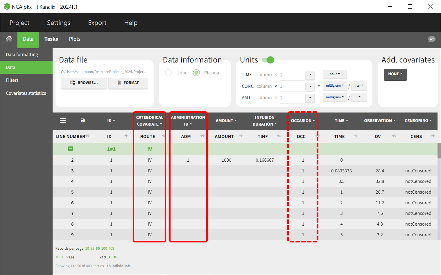
• For parallel designs, include a column distinguishing administration routes (e.g., "IV" and "PO") and tag it as a categorical covariate. An administration ID column still has to be provided to link dosing with exposure data for NCA calculations.

• For crossover designs, in addition to the administration route and administration ID columns, an occasion column has to be included to differentiate the profiles for each subject across occasions.

2. BE module configuration

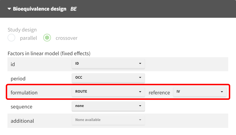
The bioequivalence module in PKanalix should be used, with the administration route assigned as a factor in the general linear model. "IV" is typically set as the reference formulation to enable group comparisons.

Methodology

The calculation employs a general linear model to determine the ratio of the geometric means of the NCA parameter e.g. AUC/dose for the different administration routes:

The GLM aggregates data for each administration route, calculating e.g. the geometric mean of the dose-normalized area under the curve (AUC/dose). This step accounts for variability between individuals and ensures a population-level comparison.
The model uses the specified factor (administration route) to partition the data into groups. Each group represents a different administration route. The GLM then fits a linear equation to the log-transformed parameter values to calculate the mean ratio between the groups.

Interpretation

The resulting average bioavailability values provide a population-level perspective:

• Higher values suggest the oral route has greater absorption efficiency compared to the intravenous (IV) route. It could be considered "high" if the value approaches or exceeds 1 (100%), as oral bioavailability typically does not surpass IV bioavailability due to factors like first-pass metabolism (where the drug being partially broken down by the liver when taken orally before reaching general circulation).

• Lower values indicate reduced absorption via the oral route. These are considered "low" when they are close to 0, indicating very poor oral bioavailability.

Incorporating interaction terms in the linear model

Introduction

Interaction terms in general linear models capture the combined effect of two variables on an outcome, reflecting how the relationship between one factor and the outcome changes depending on the modality of the other factor. For instance, a treatment-by-period interaction term reveals whether the treatment effect varies across different study periods. These terms are particularly useful in identifying dependencies or inconsistencies in study designs.

Workflow

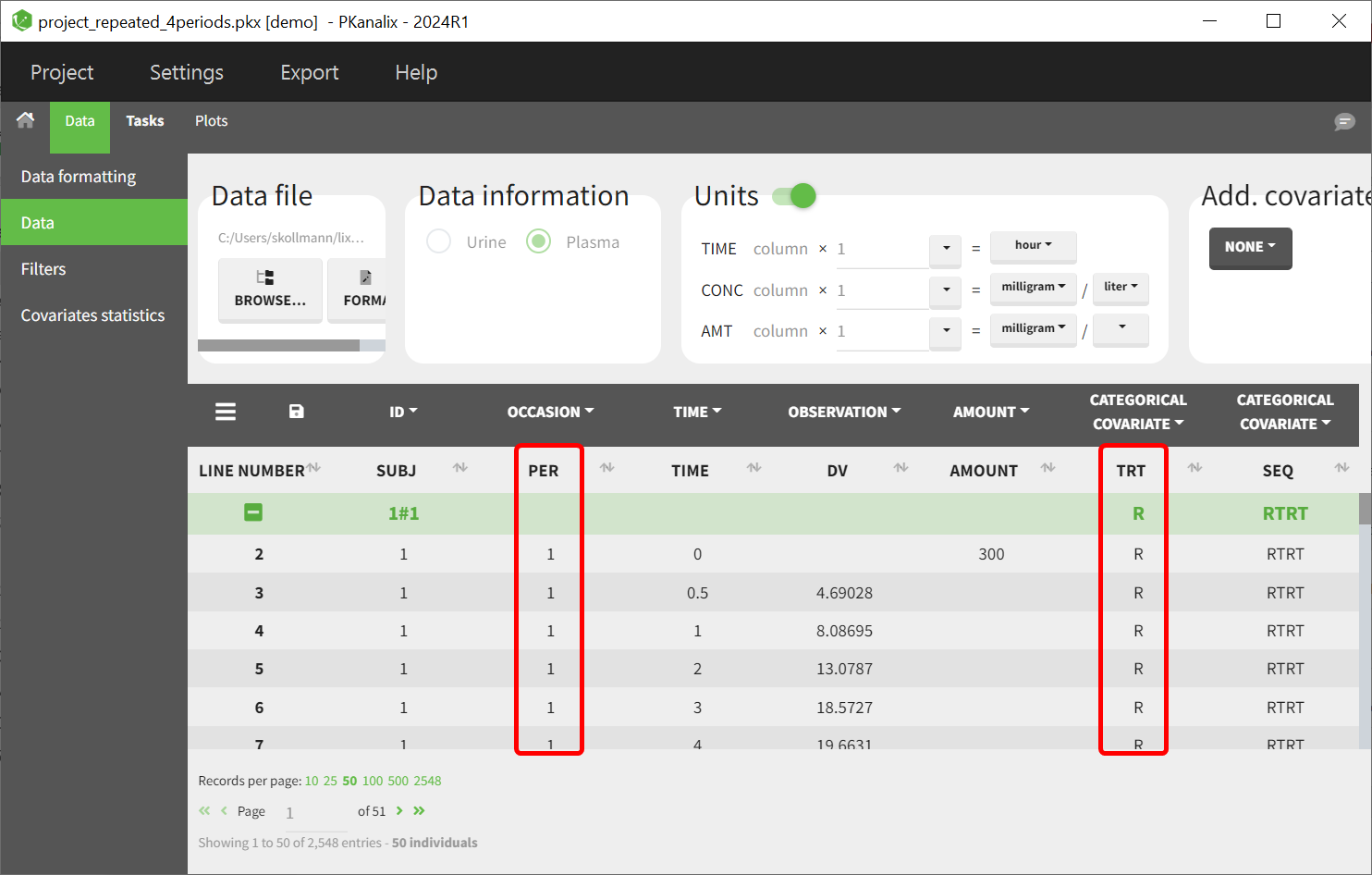
Currently, PKanalix does not natively support interaction terms in the BE module, but a workaround can be applied by creating a new "combined" covariate. The example below demonstrates this process using Period and Treatment of the demo project project_repeated_4periods.pkx as interaction variables, but the same approach applies to other variables requiring interaction analysis.

1. Identify the Variables for Interaction

Determine the two variables to be combined, such as PER and TRT. Ensure these variables are properly formatted in the dataset.

2. Create the combined covariate

Use a tool like Excel, R, or SAS to concatenate the modalities of the chosen variables into a new categorical variable. For example:

# Define the path to the Monolix Suite installation
path.software <- paste0("C:/Program Files/Lixoft/MonolixSuite2024R1")

# Uncomment the line below to install the Lixoft connectors package if not already installed
# install.packages(paste0(path.software,"/connectors/lixoftConnectors.tar.gz"), repos = NULL, type="source", INSTALL_opts ="--no-multiarch")

suppressWarnings(library(lixoftConnectors))

# Initialize the Lixoft connectors for PKanalix
initializeLixoftConnectors(software = "pkanalix", path = path.software)

# Load the demo dataset
data <- read.csv(paste0(getDemoPath(),"/3.bioequivalence/data/repeated_4periods_data.csv"),header = TRUE, sep = ",")

# Create a new column for the interaction term (e.g., Period and Treatment)
data$Interaction_Term <- paste0(data$PER, "-", data$TRT)

# Save the updated dataset to a new file
write.csv(data,"repeated_4periods_interactionterm.csv", row.names = F, quote = F)

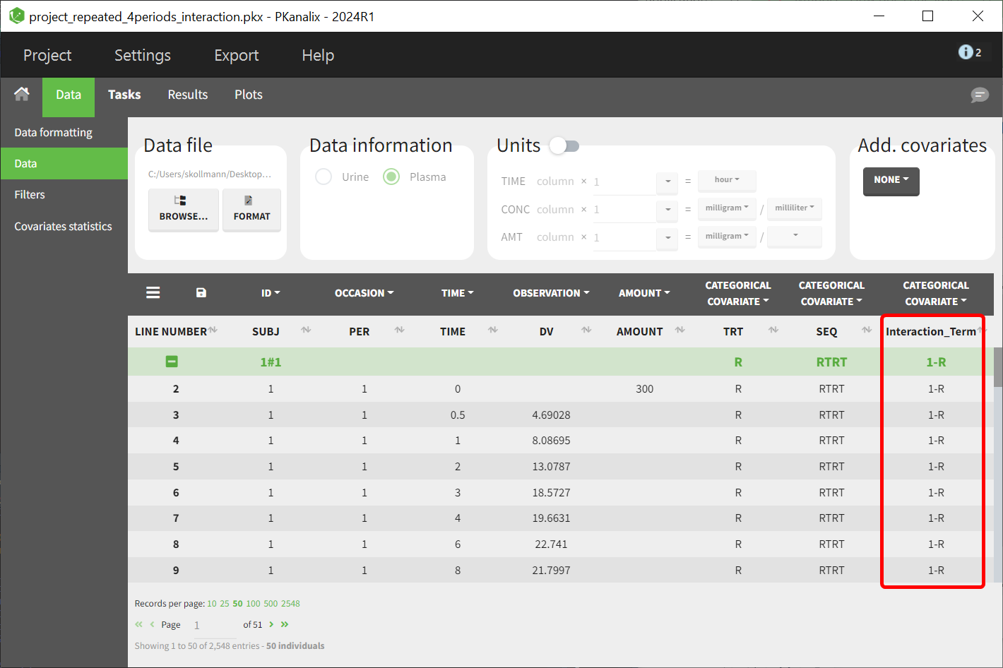
This step creates a new column (e.g., Interaction_Term) representing the interaction term.

3. Update the dataset in PKanalix

Load the updated dataset into PKanalix, ensuring the new interaction covariate is included:

4. Incorporate the combined covariate in the model

Configure the general linear model to include the new "combined" covariate as a factor for interaction analysis:

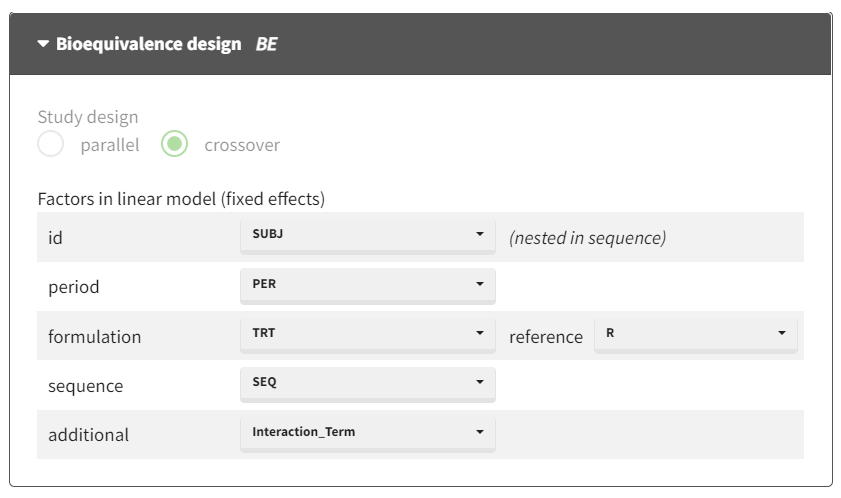
After running the model, the ANOVA table provides the breakdown of variance across factors, including the interaction term.

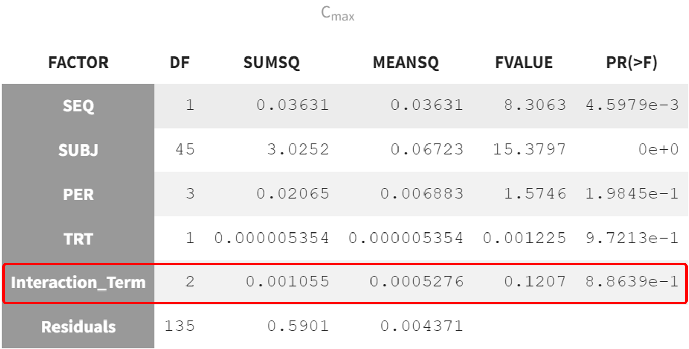
The interaction term has a p-value of 0.88639, indicating no significant interaction effect between the factors PER and TRT. This means the combined effect of these variables does not significantly impact the response, here Cmax.

Conclusion

Interaction terms offer valuable insights for detecting patterns and inconsistencies in complex datasets, especially in scenarios with heightened regulatory scrutiny. With a straightforward workaround, they can be effectively conducted in PKanalix to address specific analytical needs.