Dose linearity | MonolixSuite Documentation

Dose linearity can be described when the systemic exposure (e.g. Cmax, AUC) is a straight-line function of the administered dose amount. But unlike dose proportionality, that line need not pass through the origin. It is a weaker condition than dose proportionality: it permits a constant, dose-independent offset/intercept in exposure, so a fold change in dose does not necessarily produce the same fold change in exposure. This offset is occasionally relevant in early pharmacokinetic analysis, e.g. for endogenous compounds, where measurable exposure is present even in the absence of drug. The simple linear-model assessment described here complements the power-model dose-proportionality analysis: the power model characterises the shape of the dose–exposure relationship, while the linear model isolates its intercept [Vogel HG, Maas J, Gebauer A, editors. Drug Discovery and Evaluation: Methods in Clinical Pharmacology. Berlin, Heidelberg: Springer; 2011.].

Dose linearity linear pharamcokinetics

Dose linearity refers to the shape of the dose–exposure relationship, not to linear first-order pharmacokinetics (where rate of elimination ke conecntration). A compound can show dose-linear exposure without its clearance and volume being strictly dose-independent and vice versa. The two terms are easily confused but describe different things.

Concept and mathematics

The assessment fits a linear model by ordinary least squares, which relates a PK parameter to dose through

and focuses on the intercept . Dose proportionality is the special case . The whole assessment reduces to a single question:

Is the intercept different from zero?

This can be answered by a linear regression model along the intercept p-value: if were really 0, how often would chance alone produce an estimate this far from 0? A large p-value means the intercept cannot be told apart from 0; a small one (below the significance level, here 10%) means it is judged to differ from 0.

and p-value not significant: the intercept cannot be told apart from 0. The line passes through the origin consistent with dose proportionality.
and p-value significant: real positive offset linear but not proportional; plausible for endogenous compounds or an assay baseline.
and p-value signifcant: impossible negative exposure at dose 0 → red flag the linear assumption is wrong

The 90% confidence interval of is an equivalent check and gives the same insight: it contains 0 when the p-value is large and excludes 0 when it is small. Only the interval's position relative to 0 is informative.

Note: Linearity is assumed, not tested. Fitting a line does not verify that the relationship is a line. A saturating curve can still yield a respectable and a plausible-looking intercept.

Function `doseLinearity()`

The above explaned methodology is implemented as a single function that takes the data for one NCA parameter, retrieved by getNCAIndividualParameters()$parameters,and returns the assessment:

doseLinearity <- function(ds,                    # data set (long format)
                          parNm,                 # parameter name 
                          parVal  = "Value",     # column holding the parameter values
                          doseVal = "Dose",      # column holding the dose values
                          level   = 0.90)        # confidence level for the intercept / slope CIs
{
  # Keep only finite rows (the linear model tolerates a zero dose, but drop NA/Inf).
  ok <- is.finite(ds[[doseVal]]) & is.finite(ds[[parVal]])
  if (any(!ok))
    warning(sprintf("doseLinearity: dropping %d row(s) with non-finite values.", sum(!ok)))
  ds <- ds[ok, , drop = FALSE]
  if (length(unique(ds[[doseVal]])) < 2)
    stop("doseLinearity: need at least two distinct dose levels.")

  # Clean two-column frame so the fitted model carries tidy variable names.
  fit_df <- data.frame(param = ds[[parVal]], dose = ds[[doseVal]])

  # Linear dose-linearity model: C = alpha0 + alpha * dose.
  modlin    <- lm(param ~ dose, data = fit_df)
  smry      <- summary(modlin)
  a0.est    <- unname(coef(modlin)[1])                 # intercept  (alpha0)
  a1.est    <- unname(coef(modlin)[2])                 # slope      (alpha)
  ci        <- confint(modlin, level = level)
  a0.int    <- ci[1, ]                                 # CI of the intercept
  a1.int    <- ci[2, ]                                 # CI of the slope
  # a0.t      <- unname(smry$coefficients[1, "t value"])  # t = estimate / SE, i.e. how many SEs alpha0 sits from 0
  a0.p      <- unname(smry$coefficients[1, "Pr(>|t|)"]) # p-value of H0: alpha0 = 0 (two-sided)
  r2        <- smry$r.squared                          # goodness of the linear fit

  # Outcome of the intercept test (H0: alpha0 = 0), read off the CI / p-value.
  # a0 not significant -> line effectively through origin (consistent with, not proof of, proportionality); 
  # a0 significant -> genuine dose-independent offset.
  if (a0.int[1] <= 0 & a0.int[2] >= 0) {
    test.res <- "a0 not significant"
  } else {
    test.res <- "a0 significant"
  }
  result.tab <- data.frame(parameter          = parNm,
                           `Dosing range`     = paste0(min(ds[[doseVal]]), "--", max(ds[[doseVal]])),
                           `Intercept (a0)`   = round(a0.est, 3),
                           `Intercept CI`     = paste0("(", round(a0.int[1], 3), "; ", round(a0.int[2], 3), ")"),
                           # `t-value (a0)`     = round(a0.t, 3),
                           `p-value (a0)`     = signif(a0.p, 3),
                           `Slope (a)`        = round(a1.est, 3),
                           `Slope CI`         = paste0("(", round(a1.int[1], 3), "; ", round(a1.int[2], 3), ")"),
                           `R2`               = round(r2, 3),
                           Conclusion         = test.res,
                           check.names        = FALSE)
  # Return the tidy table; attach data, model and numeric stats as attributes.
  attr(result.tab, "data")   <- fit_df
  attr(result.tab, "modlin") <- modlin
  attr(result.tab, "stats")  <- data.frame(a0 = a0.est, a0_low = unname(a0.int[1]), a0_high = unname(a0.int[2]), a0_p = a0.p, # a0_t = a0.t, 
                                           a1 = a1.est, a1_low = unname(a1.int[1]), a1_high = unname(a1.int[2]), r2 = r2)
  result.tab
}

The core of the function is lm(param ~ dose): R's lm() fits a linear regression by ordinary least squares, i.e. it finds the intercept and slope of the straight line that best matches exposure against dose. confint() and summary() then read the 90% confidence interval and the p-value of the intercept off that fitted model.

Input data format

The function requires long-format data with one row per subject, containing (at least) a dose column and a parameter-value column. Only these two columns are used; extra columns are ignored.

id	Dose	parameter	Value
1	150	Cmax	12.3
2	150	Cmax	10.8
…	…	…	…

Point the function at the relevant columns via parVal/doseVal (defaults "Value"/"Dose"), and set the confidence level via level (default 0.90). Call it once per parameter.

Example

Using the aPCSK9_SAD.pkx PKanalix demo project, we assess dose proportionality for Cmax, AUClast and AUCINF_obs.

Via lixoftConnectors function loadProject() load the project, restrict the computed parameters to Dose, Cmax, AUClast and AUCINF_obs with setNCASettings(), run the analysis with runNCAEstimation(), and retrieve the individual NCA parameters with getNCAIndividualParameters()$parameters.

library(dplyr)
library(ggplot2)
path.software <- "C:/Program Files/Lixoft/MonolixSuite2024R1"
library(lixoftConnectors)
initializeLixoftConnectors(path.software, software = "pkanalix")
library(flextable)
##############################################################################
# helper to prepare the data
prepDataset <- function(ds,input_param){
  param <- sym(input_param)
  dt <- ds %>%
    dplyr::rename(Value=!!param)%>%
    mutate(parameter=input_param,
           Value    =as.numeric(Value))%>%
    select(id,Dose,parameter,Value)
  return(dt)
}
prj <- paste0(getDemoPath(),"/2.case_studies/project_aPCSK9_SAD.pkx")
loadProject(prj)
setNCASettings(computedNCAParameters=c("Dose","Cmax","AUClast", "AUCINF_obs"))
runNCAEstimation()
df_nca <- getNCAIndividualParameters()$parameters
df_nca <- rbind(prepDataset(df_nca, "Cmax"),
                prepDataset(df_nca, "AUClast"),
                prepDataset(df_nca, "AUCINF_obs"))

The retrieved table is in wide format (one column per parameter), so prepDataset() reshapes it into long format: one row per subject (id) and parameter, each row carrying the corresponding Dose. Once the dataset is in this format, doseProportionality() can be applied (once per parameter).

##############################################################################
# Dose linearity analysis
# Assess each parameter with the linear model; intercept judged against 0.
DL_params <- unique(df_nca$parameter)

tb.res   <- data.frame()
ci.res   <- data.frame()
stat.res <- data.frame()

for (i in DL_params){
  nca.i <- df_nca %>% filter(parameter == i)
  res.i <- doseLinearity(ds      = nca.i,
                         parNm   = i,
                         parVal  = "Value",
                         doseVal = "Dose",
                         level   = 0.90)

  tb.res <- rbind(tb.res, res.i)

  # intercept + slope + 90% CIs + R2
  st.i <- attr(res.i, "stats"); st.i$parameter <- i
  stat.res <- rbind(stat.res, st.i)

  # fitted line + 90% confidence / prediction bands (for the linear-scale plot)
  mdl.i  <- attr(res.i, "modlin")
  grid.i <- data.frame(dose = seq(min(nca.i$Dose), max(nca.i$Dose), length.out = 100))
  ci.i   <- predict(mdl.i, newdata = grid.i, interval = "confidence", level = 0.90)
  pi.i   <- predict(mdl.i, newdata = grid.i, interval = "prediction", level = 0.90)
  ci.res <- rbind(ci.res,
                  data.frame(parameter = i, Dose = grid.i$dose,
                             fit = ci.i[, "fit"],
                             ci_lwr = ci.i[, "lwr"], ci_upr = ci.i[, "upr"],
                             pi_lwr = pi.i[, "lwr"], pi_upr = pi.i[, "upr"]))
}
flextable(tb.res) %>% autofit()

Interpretation: Over the 150–800 mg dose range all three parameters return a0 not significant: although the intercept point estimates look different from 0 (e.g. roughly -100 for AUClast), their confidence intervals are wide and comfortably contain 0, so the intercept cannot be distinguished from zero. The result is consistent with dose proportionality, in agreement with the power-model assessment.

Exposure vs. dose

The linear model fit (solid), its 90% confidence interval (dashed) and 90% prediction interval (dotted) for each parameter:

ggplot(df_nca, aes(Dose, Value)) +
  geom_point(alpha = 0.6, size = 2.5) +
  geom_line(data = ci.res, aes(Dose, fit,    linetype = "Linear-model fit"),        colour = "#CD2626", linewidth = 1.2) +
  geom_line(data = ci.res, aes(Dose, ci_lwr, linetype = "90% confidence interval"), colour = "#1874CD", linewidth = 1.1) +
  geom_line(data = ci.res, aes(Dose, ci_upr, linetype = "90% confidence interval"), colour = "#1874CD", linewidth = 1.1) +
  geom_line(data = ci.res, aes(Dose, pi_lwr, linetype = "90% prediction interval"), colour = "#008B45", linewidth = 1.0) +
  geom_line(data = ci.res, aes(Dose, pi_upr, linetype = "90% prediction interval"), colour = "#008B45", linewidth = 1.0) +
  scale_linetype_manual(name   = NULL,
                        breaks = c("Linear-model fit", "90% confidence interval", "90% prediction interval"),
                        values = c("Linear-model fit"         = "solid",
                                   "90% confidence interval"  = "dashed",
                                   "90% prediction interval"  = "dotted")) +
  expand_limits(x = 0) +  
  guides(linetype = guide_legend()) +
  facet_wrap(~ parameter, scales = "free_y") +
  labs(x = "Dose", y = "Parameter value") +
  theme_bw()

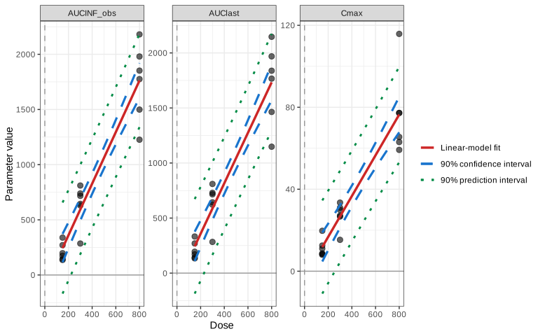
Over the 150–800 mg range the observations fall close to the fitted line with a good fit, and when the line is extrapolated back to dose 0 it meets the axis approximatively at the zero-exposure line for Cmax and only below it for AUClast and AUCINF_obs.

Intercept vs. zero (decision plot)

The intercept estimate (point estimate) and its 90% confidence interval

intercept_a0 <- ggplot(stat.res, aes(x = a0, y = factor(parameter, levels = DL_params))) +
  geom_vline(xintercept = 0, linetype = "dotted", linewidth = 0.6) +
  geom_errorbar(aes(xmin = a0_low, xmax = a0_high), width = 0.15) +
  geom_point(size = 2.5) +
  annotate("text", x = 0, y = Inf, label = "Intercept = 0", vjust = 1.4, fontface = "bold", size = 3.2) +
  labs(x = expression(alpha[0] ~ "(intercept) with 90% CI"), y = NULL) +
  theme_bw() +
  theme(panel.grid  = element_blank(),
        plot.title  = element_text(hjust = 0.5, face = "bold"),
        plot.margin = margin(t = 18, r = 12, b = 6, l = 6))

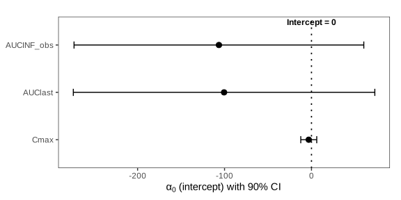
Each point estimates confidence interval contains 0 (crosses the “Intercept = 0” line). For all three parameters the intercept cannot be distinguished from zero consistent with dose proportionality.

Last updated: July 15, 2026

Dose linearity \ne linear pharamcokinetics