Basic Simulx workflow

Load a project and run the simulation

Simple example to load an existing project, run the simulation and look at the results:

R

# load and initialize the API
library(lixoftConnectors) 
initializeLixoftConnectors(software="simulx")

# Get the project
project <- paste0(getDemoPath(), "/2.models/longitudinal.smlx")
loadProject(projectFile = project)

# Run the simulation
runSimulation()

# The results are accessible through the function getSimulationResults()
# The results for the output is the list res and TS is one of the outputs
head(getSimulationResults()$res$TS)

  id time       TS
1  1    0 10.00000
2  1    1 11.04939
3  1    2 12.20862
4  1    3 13.48915
5  1    4 14.90359
6  1    5 16.46585

Import a Monolix project and simulate a new output variable with the EBEs

https://www.youtube.com/watch?v=7DzzWzQ5XdM

In this example, the Monolix demo theophylline_project.mlxtran is imported to Simulx. A new variable AUC is added to the model, and it is simulated on a regular grid using the EBEs estimated in the Monolix project. This requires that the tasks “Population parameters” and “EBEs” have run in the Monolix project.

R

# Import a Monolix project and simulate a new output variable with the EBEs  =====
# Load and initialize library =====
library(lixoftConnectors)
initializeLixoftConnectors(software = "monolix")

#Load project from Monolix Demos and run it to get EBEs estimated =====
MonolixProject <- paste0(getDemoPath(), "/1.creating_and_using_models/1.1.libraries_of_models/theophylline_project.mlxtran") 
loadProject(MonolixProject) 
runScenario() 
initializeLixoftConnectors(software = "simulx", force = TRUE) 

#IMPORT Monolix project and check that mlx_EBEs element has been created =====
importProject(MonolixProject) getIndividualElements() 

#SET ADDITIONAL formula in the model to compute the AUC =====
setAddLines("ddt_AUC = Cc") # define a new element output with a regular grid for the variable "AUC" 
defineOutputElement(name="AUCregular", element = list( data = data.frame( start = 0, interval = 1, final = 120), output = "AUC")) 
#CHECK the simulation group that already exists =====
getGroups() 
# => we currently have one group, called "simulationGroup1", which uses the following elements:
# - mlx_Pop (population parameter values) => need to be replaced by mlx_EBEs
# - mlx_Adm1 (treatment from monolix data set) => OK
# - mlx_CONC (output CONC with times as in monolix data set) => need to be replaced by AUC with new grid
# - size = 12 (same number of in original data set) => OK

#MODIFY the existing simulation group such that it uses EBEs and the new output element=====
setGroupElement(group = "simulationGroup1", 
                elements = c("mlx_EBEs", "AUCregular"))

# check the new simulation setup
getGroups()

#Set shared IDs to say the individuals in the treatment element and in the parameter element are the same and should alwyas be sampled together =====
setSharedIds(c("treatment","individual"))

# check the simulation setup
getGroups()
getSharedIds()

# - mlx_EBEs => ok
# - remaining parameters (error model parameters if residual error is simulated) => not needed as we output model predictions
# - mlx_Adm1 => ok
# - AUCregular => ok
# - size=12 => ok


#SAVE and RUN project =====
saveProject("simulx_api_example.smlx")

# run simulation
runSimulation()


#GET the results: simulated values for AUC and sampled individual parameters =====
simulatedParam <- getSimulationResults()$IndividualParameters$simulationGroup1
simulatedOutput <- getSimulationResults()$res$AUC


#PLOT the results =====
library(ggplot2)
ggplot(data = simulatedOutput, aes(x=time, y=AUC))+
  geom_line() + aes(color = factor(as.double(original_id)))+
  labs(colour="Original ID")

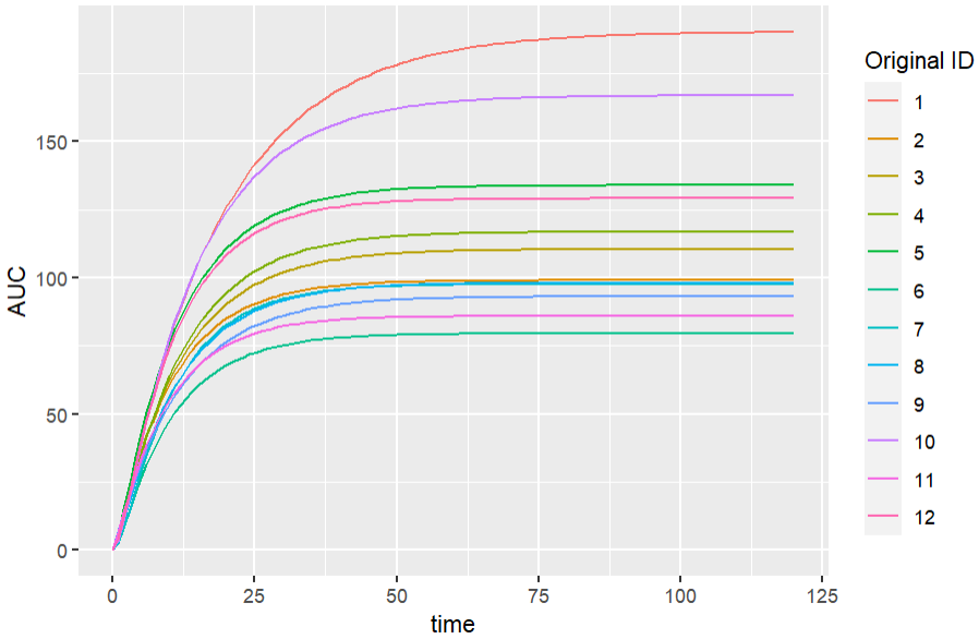
We get the following simulations for the new output variable. “Original_id” is the ID used in the original dataset loaded in the Monolix project.

Create a Simulx project from scratch and simulate covariate-dependent treatments

This script creates a project similar to the demo project treatment_weight_and_genotype_based.smlx, available in the folder 3.1.treatments of Simulx demos. The model file TMDDmodel.txt can be downloaded here: TMDDmodel.txt.

While in the interface of Simulx it is possible to directly define distribution laws for covariates and covariate-dependent treatments that are computed at the simulation step, in R it is necessary to sample covariates from distributions and derive the corresponding doses before defining the elements for the simulation.

R

###############################################################
# Create a Simulx project from scratch and simulate covariate-dependent treatments
###############################################################

# load and initialize the API 
library(lixoftConnectors) 
initializeLixoftConnectors(software = "simulx")

# Create a new project based on the model
newProject(modelFile = "TMDDmodel.txt")

# Define vector of population parameters
definePopulationElement(name="PopParameters", 
                        element = data.frame(V_pop=3, omega_V=0.1 ,Cl_pop=0.1, omega_Cl=0.1, Q_pop=1, omega_Q=0.2,
                                             V2_pop=3, omega_V2=0.2, beta_V_logtWeight=1, KD_pop=0.01, omega_KD=0.01,
                                             R0_pop=0.2, omega_R0=0.3, kint_pop=50, omega_kint=0.2, kon_pop=10,
                                             omega_kon=0.01, ksyn_pop=10, omega_ksyn=0.2, beta_Cl_logtWeight=0.75,
                                             beta_Q_logtWeight=0.75, beta_V2_logtWeight=0.75, 
                                             beta_KD_Genotype_Heterozygous=1.3))

# Define covariates: in the interface it is possible to define distribution laws,
# but in R we have to sample from the distributions prior to the simulation.
# Here we define 3 tables for the 3 simulation groups
for (i in 1:3){
  covTable <- data.frame(id=1:250,
                         Weight = rlnorm(n=250, mean=log(70), sd=0.3),
                         Genotype=c("Homozygous", "Heterozygous")[sample(1:2, 250, replace=T)])
  write.csv(covTable, file = paste0("covTable",i,".csv"), quote=F, row.names=F)
  defineCovariateElement(name=paste0("covTable",i),
                         element = paste0("covTable",i,".csv"))
}

# Define common treatment
defineTreatmentElement(name="1000nmol", element=list(admID=1, data=data.frame(time=seq(0,by=21,length.out = 5), 
                                                                              amount=1000, tInf=0.208)))

# Define weight-based treatment: in the interface it can be done directly with a scaling formula,
# but in R we have to define a table of individual doses prior to the simulation.
# We use covTable2.csv for simulation group 2.
covTable <- read.csv("covTable1.csv")
trt_14nmolPerKg <- data.frame(id=rep(1:250, each=5),
                              time=rep(seq(0,by=21,length.out = 5), times=250),
                              amount=14*covTable$Weight, tInf = 0.208)
write.csv(trt_14nmolPerKg, file="trtTableWeight.csv", quote=F, row.names=F)
defineTreatmentElement(name="14nmolPerKg", element=list(admID=1, data="trtTableWeight.csv"))

# Define genotype-based treatment: in the interface it can be done directly with a scaling formula,
# but in R we have to define a table of individual doses prior to the simulation.
# We use covTable3.csv for simulation group 3.
covTable <- read.csv("covTable3.csv")
trt_genotype <- data.frame(id=rep(1:250, each=5),
                           time=rep(seq(0,by=21,length.out = 5), times=250),
                           amount=ifelse(covTable$Genotype=="Heterozygous", 1000, 800), tInf = 0.208)
write.csv(trt_genotype, file="trtTableGenotype.csv", quote=F, row.names=F)
defineTreatmentElement(name="1000nmolHomo_800nmolHetero", element=list(admID=1, data="trtTableGenotype.csv"))

# Define outputs
defineOutputElement(name="Concentration", element = list(output="L", data=data.frame(time=seq(0,96,by=1))))
defineOutputElement(name="TargetOccupancy", element = list(output="TO", data=data.frame(time=seq(0,96,by=1))))

# By default there is a single simulation group named simulationGroup1,
# change its name and set all elements for the simulation
setGroupSize("simulationGroup1", 250)
setGroupElement("simulationGroup1", elements = c("PopParameters","14nmolPerKg","Concentration","TargetOccupancy", "covTable1"))
renameGroup("simulationGroup1", "Weight_based")

# Define the two other simulation groups with different covariates and treatments.
# By default the other elements are the same as the first group
addGroup("Flat_dose")
setGroupElement("Flat_dose", elements = c("1000nmol","covTable2"))
addGroup("Genotype_based")
setGroupElement("Genotype_based", elements = c("1000nmolHomo_800nmolHetero","covTable3"))

# Save project and run the simulation
saveProject(projectFile = "treatment_weight_and_genotype_based.smlx") 
runSimulation()

# Get simulation results: a table of individual parameters for each group, and a table of simulated values for each output
sim <- getSimulationResults()
names(sim$IndividualParameters) # "Weight_based", "Flat_dose", "Genotype_based"
names(sim$res) # "L", "TO"

Import a Monolix project and simulate with new output times

Monolix simulates the original dataset with replicates to generate the VPC. It can be useful to perform the same simulations in Simulx with modified observation times, for example to correct the bias in VPC due to dropout. The example below shows this step, and uses the project PDTTE_dropout. The full example to correct a VPC for dropout is detailed on this page.

In this example the Monolix project with the biased VPC is named PD_TTE.mlxtran, the new regular measurement times are similar to the measurements in the original dataset, but are not impacted by dropout, and the number of replicates is 500 (as the default number of simulations for the VPC in Monolix). The random variable capturing dropouts in the model used in Monolix is called survival.

R

###############################################################
# Import a Monolix project and simulate with new output times
###############################################################

library(lixoftConnectors)
initializeLixoftConnectors(software = "simulx")

importProject(projectFile = "PDTTE_dropout.mlxtran")
defineOutputElement(name="y1_alltimes", element = list(output="y1", data=data.frame(time=seq(-100,1500,by=100))))
setGroupElement("simulationGroup1", elements = c("y1_alltimes","mlx_survival"))
setNbReplicates(500) 
saveProject(projectFile = "PD_TTE_alltimes.smlx")
setPreferences(exportsimulationfiles=T)
runSimulation()