For complex PKPD models it can be difficult to understand the contribution of each parameter to the model outputs. In such cases a sensitivity analysis can be a powerful way to investigate which parameter will have the biggest influence.
A sensitivity analysis can be performed with the R package sensitivity.
Sensitivity analysis for longitudinal data should be based on an unidimensional summary of the data, such as the integral, i.e. the area under the curve (AUC), the minimum or the maximum value over an interval, for instance. Such quantities can be computed with the Simulx and PKanalix functions of the lixoftConnectors package.
Combining the packages lixoftConnectors and sensitivity is therefore a powerful solution for sensitivity analysis of PKPD models.
library(sensitivity)
library(lixoftConnectors)
We will consider a basic one-compartement PK model for oral administration. The sensitivity analysis will be based on the exposure at steady state, when repeated doses of 5 mg are given every 12 hours.
The model and the design are defined in a Simulx project (project.zip) and we create a function sensModel which returns NCA metrics (such as AUC, Cmax or Tmax) according to the parameter values used for the sensitivity analysis.
The PK parameters ka, V and k are the input arguments of this function.
sensModel <- function(x){
  initializeLixoftConnectors("simulx", force = TRUE)
  loadProject(project)

  df_params <- as.data.frame(x)
  names(df_params) <- names
  df_params <- cbind(data.frame(id=1:nrow(df_params)), df_params)
  file <- tempfile(pattern = "file", fileext = ".csv")
  write.csv(df_params, file, row.names = FALSE)
  defineIndividualElement(name = "parameters", element = file)

  setGroupElement("simulationGroup1", "parameters")
  setGroupSize("simulationGroup1", nrow(df_params))
  runSimulation()

  exportProject(settings = list(targetSoftware = "pkanalix"), force = TRUE)
  setNCASettings(computedNCAParameters = metric)
  runNCAEstimation()

  if (length(metric) > 1)
    return(getNCAIndividualParameters()$parameters)
  else
    return(getNCAIndividualParameters()$parameters[[metric]])
}
If we want to see, for instance, the impact of ka on the exposure at steady state, we can use this function with two different sets of PK parameters (ka=0.2, V=10, k=0.2 and ka=0.5, V=10, k=0.2) and return the output by setting metric to c("AUClast", "Cmax", "Tmax").
project <- "project.smlx"
metric <- c("AUClast", "Cmax", "Tmax")
names <- c("ka", "V", "k")

r <- sensModel(matrix(c(0.2,0.5,10,10,0.2,0.2), nrow=2))
print(r)

#>   id  AUClast     Cmax Flag_Lambda_z_Rule Tmax
#> 1  1 2.499917 0.257020                  1  3.8
#> 2  2 2.499791 0.317503                  1  2.7
We can see that changing the value of ka from 0.2 to 0.5 doesn’t modify the area under the curve (AUClast) but impacts the time at which the maximum concentration is observed (Tmax).
For a more exhaustive sensitivity analysis, let us use now the fast99 function which implements the so-called extended-FAST method (Saltelli et al. 1999).
Here, ka takes its values between 0.2 and 0.5, V between 5 and 10, and k between 0.05 and 0.1.
Sensitivity analysis is first based on AUC.
l1 <- list(min = 0.2, max = 0.5)
l2 <- list(min = 5, max = 10)
l3 <- list(min = 0.05, max = 0.1)

metric <- "AUClast"
x <- fast99(model = sensModel, factors = 3, n = 500,
            q = "qunif", q.arg = list(l1,l2,l3) )
print(x)

#> Call:
#> fast99(model = sensModel, factors = 3, n = 500, q = "qunif",     q.arg = list(l1, l2, l3))
#>
#> Model runs: 1500
#>
#> Estimations of the indices:
#>     first order total order
#> X1 2.271657e-06  0.00224729
#> X2 4.878211e-01  0.51200394
#> X3 4.878359e-01  0.51201873
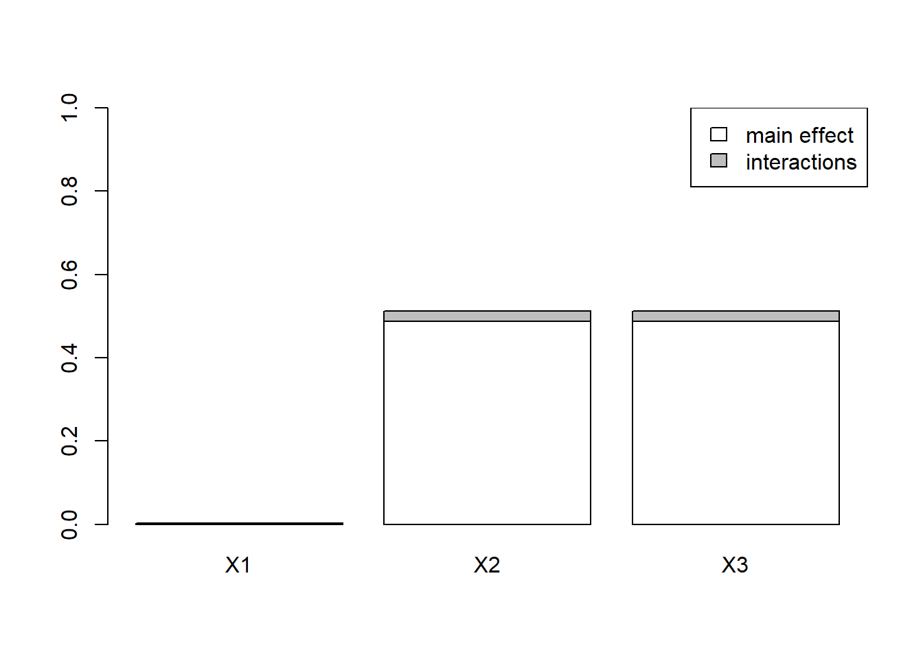
plot(x)

Sobol indices measure the contributions of each PK parameter to the variability of AUC. A Sobol index of zero means that the variance of the parameter has no contribution on the variance of the output and a Sobol index of one means that the variance in the output is 100% dependent on the variance of the parameter.
This index is almost 0 for ka but is significantly different from 0 for both V and k.
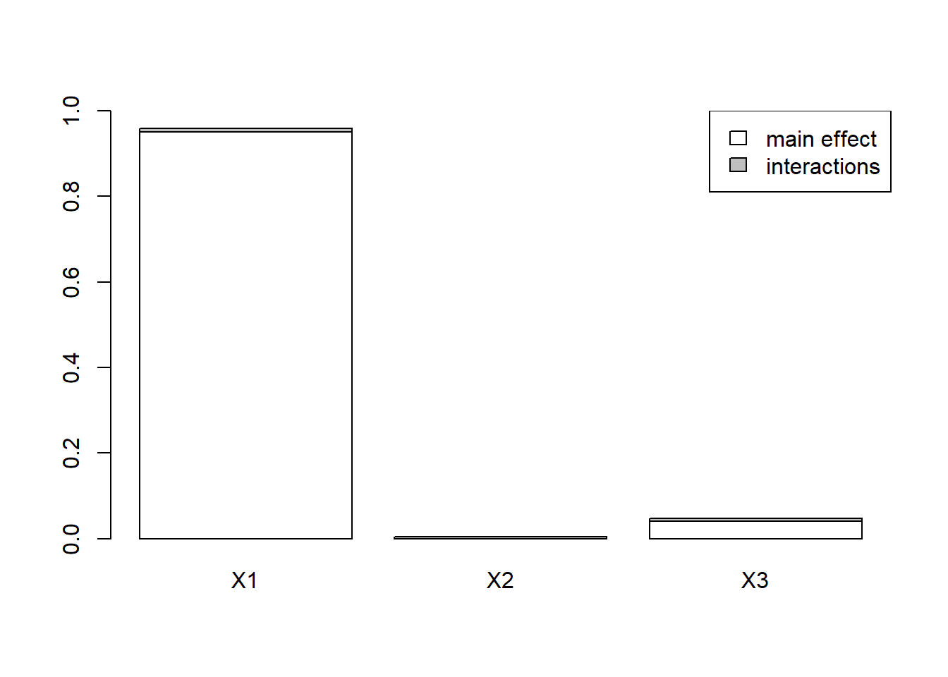
If we now use Tmax instead of AUC for our sensitivity analysis, we see that it’s ka which explains almost all the variability of Tmax.
metric <- "Tmax"
x <- fast99(model = sensModel, factors = 3, n = 500,
            q = "qunif", q.arg = list(l1,l2,l3) )
print(x)

#> Call:
#> fast99(model = sensModel, factors = 3, n = 500, q = "qunif",     q.arg = list(l1, l2, l3))
#>
#> Model runs: 1500
#>
#> Estimations of the indices:
#>     first order total order
#> X1 0.9501601980 0.958651102
#> X2 0.0001179046 0.003735798
#> X3 0.0414159525 0.047826852
plot(x)

Several methods are available in the package sensitivity. sobolEff implements the Monte Carlo estimation of the Sobol’ sensitivity indices using the asymptotically efficient formulas in section 4.2.4.2 of Monod et al. (2006).
We need a function that randomly draws PK parameters uniformly distributed in given intervals.
mySim <- function(r, n){
  M <- length(r)
  X <- data.frame(matrix(runif(M * n), nrow = n))
  for (m in (1:M)) {
    rm <- r[[m]]
    X[,m] <- X[,m]*(rm$max-rm$min) + rm$min
  }
  return(X)
}
Monte Carlo methods for estimating the Sobol indices use two random samples X1 and X2 of the PK parameters.
X1 <- mySim(list(l1,l2,l3), n=200)
X2 <- mySim(list(l1,l2,l3), n=200)
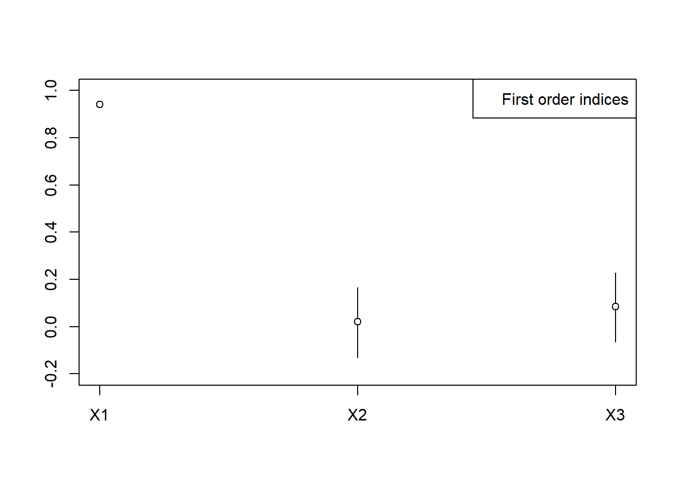
x <- sobolEff(model=sensModel, X1=X1, X2=X2, order=1, nboot=500)
print(x)

#> Call:
#> sobolEff(model = sensModel, X1 = X1, X2 = X2, order = 1, nboot = 500)
#>
#> Model runs: 800
#>
#> Model variance: 0.1266477
#>
#>
#>
#> Sobol indices
plot(x, ylim=c(-0.2, 1))

References
-
[Package “sensitivity”] (http://cran.r-project.org/web/packages/sensitivity/sensitivity.pdf)
-
A. Saltelli, S. Tarantola and K. Chan, 1999, A quantitative, model independent method for global sensitivity analysis of model output, Technometrics, 41, 39-56.
-
Monod, H., Naud, C., Makowski, D. (2006), Uncertainty and sensitivity analysis for crop models in Working with Dynamic Crop Models: Evaluation, Analysis, Parameterization, and Applications, Elsevier.

