Vanoxerine: identification of a delay

Original data

This C-QTc case study is based on a clinical trial data of a human laboratory study of Vanoxerine (GBR 12909) – a dopamine uptake inhibitor developed to treat cocaine dependence.

The clinical study was a double-blind, placebo-controlled, dose-escalating trial designed to assess the safety, tolerance, and pharmacokinetics of multiple escalating doses of Vanoxerine in cocaine-experienced volunteers.

The original study involved three escalating oral doses of Vanoxerine, administered daily for 10 days. Participants were divided into treatment and placebo groups, with two individuals receiving placebo. Drug concentration (mg/L) was measured starting after the third dose and QT interval measurements were collected for all participants.

The data was obtained from the National Institute on Drug Abuse (NIDA) database at NIDA-CPU-0002 study. The plasma GBR12909 concentration is obtained from the EXTLABS.csv file, the ECG data from the ECGPRFL1.csv file and the treatment groups from the RDMCODE.csv file. The following R code is used to read and merged this information into a single file.

library(dplyr)
# read placebo and treatment groups (50 or 75 mg)
# remove placebo individuals and individuals that did not meet inclusion criteria
TRT <- read.csv("../ascii-crf-files_nida-cpu-0002/RDMCODE.csv") %>%
  filter(XTRTMT!="" & XTRTMT!="Placebo") %>%
  select(c(SUBJID,XTRTMT))
# read ECG data
ECG <- read.csv("../ascii-crf-files_nida-cpu-0002/ECGPRFL1.csv") %>% 
  select(c(STUDYID, SUBJID, VISID, ECGHOUR, ECG12TM, ECGPR, ECGQT, ECGQRS, ECGRR)) %>%
  group_by(SUBJID, VISID) %>%
  mutate(TIME=c(0, 0.5, 1, 2, 3, 4, 6, 8, 12)) %>%                 # add time column (nominal times based on protocol)
  mutate(BASELINE=if_else(TIME==0,"Y","N")) %>%                    # add baseline column (Y or N)
  mutate(TRT=if_else(VISID=="DAY0","Placebo","Vanoxerine")) %>%    # add treatment column with "placebo" or "vanoxerine"
  ungroup() %>%
  right_join(TRT, by="SUBJID")                                     # keep only non-placebo individuals using right_join
# read concentration data
CONC_ngmL <- read.csv("../ascii-crf-files_nida-cpu-0002/EXTLABS.csv") %>% 
  filter(TESTNAME=="Plasma GBR Concentration") %>%    # keep only PK measurements
  filter(COLLDATE==11) %>%                            # keep only day 11 (only troughs on the other days)
  right_join(TRT, by="SUBJID") %>%                    # keep only non-placebo individuals using right_join
  filter(!(SUBJID=="284255" & TIMETEXT==758)) %>%     # remove one duplicate conc for this id
  group_by(SUBJID) %>%
  mutate(TIME=c(0, 0.5, 1, 1.5, 2, 2.5, 3, 4, 6, 8, 12)) %>% # nominal times based on protocol (more points for CONC compared to QTc)
  mutate(VISID="DAY11") %>%
  select(c(SUBJID,VISID,TIME,RESULT)) %>%
  rename(CONC = RESULT) %>%
  ungroup()
# merge ECG and conc data
ECG_CONC <- ECG %>% 
  left_join(CONC_ngmL, by=c("SUBJID","VISID","TIME")) %>%  # merge conc data
  mutate(CONC=if_else(VISID=="DAY0","0",CONC)) %>%         # put conc = 0 for day 0 (placebo)
  mutate(TRT = if_else(TRT=="Placebo","Placebo",if_else(XTRTMT=="GBR12909 50 mg", "Vanoxerine 50 mg", "Vanorexine 75 mg"))) %>%
  rename(VISIT=VISID, DOSEGROUP=XTRTMT)%>%
  select(c(STUDYID, SUBJID, VISIT,TRT, TIME, CONC, BASELINE, ECGPR, ECGQT, ECGQRS, ECGRR))
write.csv(ECG_CONC, file="Vanoxerine_data.csv", quote=F, row.names = F)

We obtain the following dataset structure:

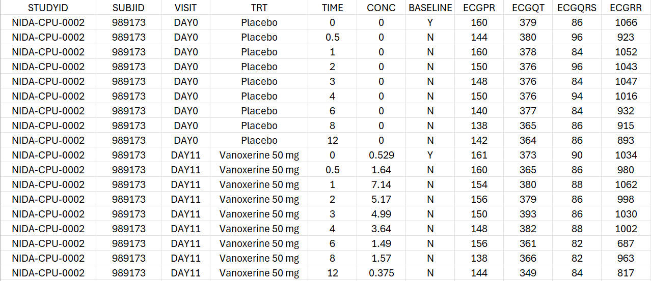
For each individual, the concentration and the PR, QT, QRS and RR intervals are measured on Day 0 under placebo treatment and on Day 11 under active treatment with either 50 mg or 75 mg of vanoxerine. For each period, the observations are recorded at time 0, 0.5, 1, 2, 3, 4, 6, 8 and 12 hours post-dose.

Data formatting

In order to perform a concentration-QTc analysis and generate exploratory data analysis plots, it is necessary to apply the following processing steps:

• calculate heart-rate correction for QT to generate QTc, for instance using Fridericia’s formula

• calculate the baseline-corrected QTc, i.e ΔQTc. In our case, the baseline is simply the pre-dose measurement at time 0 hr. It is indicated in the dataset with BASELINE=Y

• given that both placebo and vanoxerine periods are available for each individual, it is also possible to calculate directly the baseline-corrected and placebo-corrected QTc, i.e ΔΔQTc

• for exploratory data visualization purpose, the ΔHR and ΔΔHR can also be computed

Covariates and regressor variables which will appear in the conc-QTc model must also be added as additional columns:

• BLQTc_cent: the centered QTc baseline

• BLQTc_centAdjPl: the placebo-adjusted centered baseline in case of ΔΔQTc

• TIME_cat: time as categorical factor

• Cc_reg: drug concentration

• RR_reg: RR interval duration (for plotting purpose)

These steps can be performed using the function process_QTcData().

First, the R script mlxQTcTools.R , which contains the conc-QTc related functions, must be sourced. In addition, to use these R functions, a MonolixSuite installation must be available and the lixoftConnectors R package installed. In order to indicate the location of the MonolixSuite installation, the functioninitQTc(path=...) is used.

source('../_mlxQTcTools/mlxQTcTools.R')
initQTc(path="C:/Program Files/Lixoft/MonolixSuite2024R1")

The process_QTcData() is called in the following way:

process_QTcData(data = "Vanoxerine_data.csv", 
                QTname = "ECGQT", RRname = "ECGRR", CONCname = "CONC", 
                TRTname = "TRT", IDname = "SUBJID", TIMEname = "TIME", 
                placeboName = "Placebo",
                bComputeBaseline = TRUE, BLFLAGname = "BASELINE", baselineType = "predose",
                bComputeQTc = TRUE, correctionMethod = "Fridericia", 
                outName = "Vanoxerine_formatted.csv", silent = FALSE)

The column containing the QT, RR, drug concentration, treatment (placebo or drug), subject id and time are indicated using the arguments QTname, RRname, CONCname, TRTname, IDname, TIMEname. Note that the values present in the TRTname column will be used as plot labels for the report generation. If several dose levels are used, the TRTname column should contain different values for the different dose levels, for instance “Placebo”, “Vanoxerine 50 mg” and “Vanoxerine 75 mg”.

Given that the QTc column (heart rate-corrected QT) is not present in the dataset, it is computed using bComputeQTc = TRUE. Several correction methods are available and can be chosen. To use the most common Fridericia formula, we set correctionMethod = "Fridericia".

The QTc baseline column is not present yet in the dataset, so it is computed by setting bComputeBaseline = TRUE and indicating the baseline flag column in BLFLAGname. The baseline flag column should contain “0”/”1” values or “N”/”Y” values with “Y” and “1” indicating the baseline records.

The name of the output file is given via the outName argument.

Running the function generates the following console output, which details the applied formatting steps. This output can be supressed by choosing silent=T.

Info: The following treatment groups have been found: Placebo, Vanoxerine 50 mg, Vanorexine 75 mg
Info: The HR column has not been provided and has been calculated based on the 'ECGRR' column.
Info: The QTc column has been calculated based on the 'ECGQT' and 'ECGRR' columns, using Fridericia's formula: QTc=QT/(RR/1000)^(1/3)
Info: The BLQTc and BLHR columns have been calculated using the lines flagged as BASELINE=Y or 1.
Info: The dQTc and dHR columns have been calculated as dQTc=QTc-BLQTc and dHR=HR-BLHR.
Info: The BLQTc_cent column has been calculated as BLQTc_cent=BLQTc-mean(BLQTc).
Info: The ddQTc, ddRR and BLQTc_centAdjPl columns have be computed by subtracting the placebo data. 
Info: The Cc_reg (concentration as regressor), RR_reg (RR as regressor) and TIME_cat (TIME as categorical covariate) columns have been added.
 ==> Created new dataset Vanoxerine_formatted.csv. 

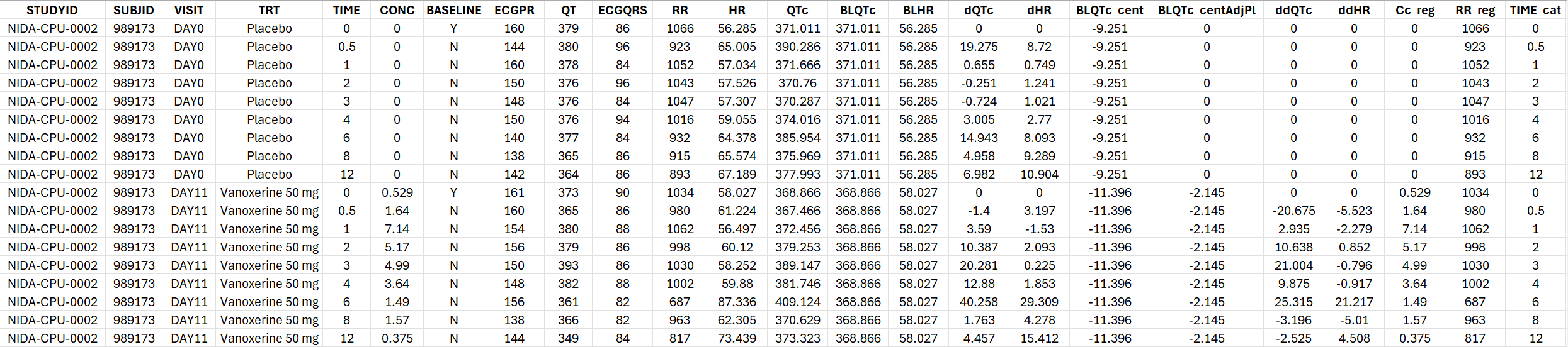
The generated formatted dataset has the following structure:

Linear model fitting

Given that placebo data is available for each individual, ΔΔQTc can be calculated and modeled directly.

To run a C-QTc analysis for ΔΔQTc with the standard linear model, the function generateQTcProject() can be used:

generateQTcProject(dataSet="Vanoxerine_formatted.csv", 
                   IDname="SUBJID", TIMEname="TIME", TRTname="TRT", CONCname="CONC", 
                   placeboName = "Placebo", 
                   modelFile = "../_mlxQTcTools/models/ddQTcModels/model_ddQTc_Linear.txt", 
                   projectName = "./mlx_runs_linearOnly/ddQTc_Linear.mlxtran", 
                   isddQTC = TRUE, 
                   bRun = TRUE)

The user should provide the formatted dataset in the argument dataSet, as well as the name of the columns containing the subject id in IDname, time in TIMEname, treatment groups in TRTname, concentration in CONCname. The other columns (e.g QT, QTc, HR, etc) must have predefined headers and do not need to be specified. The category of the treatment group column representing placebo can be indicated using placeboName = "Placebo".

To select the standard linear model for ΔΔQTc, the file model_ddQTc_Linear.txt from the model library provided with the R functions can be used. The Monolix project will be saved as projectName = "./mlx_runs_linearOnly/Vano_standard_model.mlxtran".

Whether ΔΔQTc or ΔQTc is used must be indicated with isddQTC = T or F. To run the projects, use bRun = T. Given that each individual has a placebo period and ΔΔQTc could be computed, we model directly ΔΔQTc, which allows for faster runs.

Report generation

The following assumptions should be assessed to decipher the applicability of the standard linear model:

• Assumption 1: No drug effect on HR

• Assumption 2: QTc interval is independent of HR

• Assumption 3: No time delay between drug concentrations and ΔQTc or ΔΔQTc

• Assumption 4: Linear C-QTc relationship

Exploratory data analysis plots can be generated to assess these assumptions. This can be done via the generation of a report in Word format, based on a Quarto template. A Quarto template is provided as part of the R functions and can be used in the following way:

quarto_render(input = "../_mlxQTcTools/QTc_quarto_allModels.qmd", 
              output_file = "Vanoxerine_ddQTc_report.docx",
              execute_params = list(folderName = "../Example_Vanoxerine/mlx_runs",   # give relative path from quarto template (.qmd) to folder containing runs
                                    compoundName = "Vanoxerine",
                                    CONCcolumn = "CONC", 
                                    TRTcolumn = "TRT",
                                    bHasPlacebo = TRUE,
                                    placeboName = "Placebo", 
                                    studyType = "ddQTc",
                                    concentrationUnit = "ng/mL",
                                    nBins = 10,
                                    orderTRT = c("Placebo","Vanoxerine 50 mg", "Vanorexine 75 mg"),
                                    thresBICc = 0))

The input argument give the path to the Quarto template, while the output_file is the generated Word report. The folderName gives the relative path from quarto template (.qmd) to folder containing the Monolix runs. Note that it is not the relative path from the current working directory but from the Quarto template. The compoundName and concentrationUnit will be used in the text and plot labels of the report, while placeboName should be the category of the treatment column representing the placebo individuals. The studyType can be dQTc (for ΔQTc) or ddQTC (for ΔΔQTc). The number of bins nBins will be applied in plots when binning of the concentration values is necessary.

The key diagnostic plots contained in the report are presented below. The entire report can be downloaded here and visualized below.

A selection of diagnostic plots is shown below.

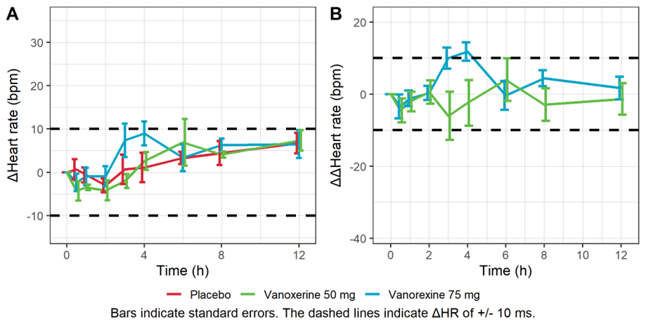
Assumption 1: No drug effect on HR

The figure below shows the time course of the mean heart rate stratified by treatment to assess a potential drug effect on heart rate. Although there is no consensus on the specific threshold effect on HR that could influence QT/ QTc assessment, mean changes of 10 bpm or more are considered problematic. The figure shows no significant effect of the drug concentration on ΔHR or ΔΔHR.

Mean baseline corrected (A) and baseline- and placebo-corrected (B) heart rate vs time.

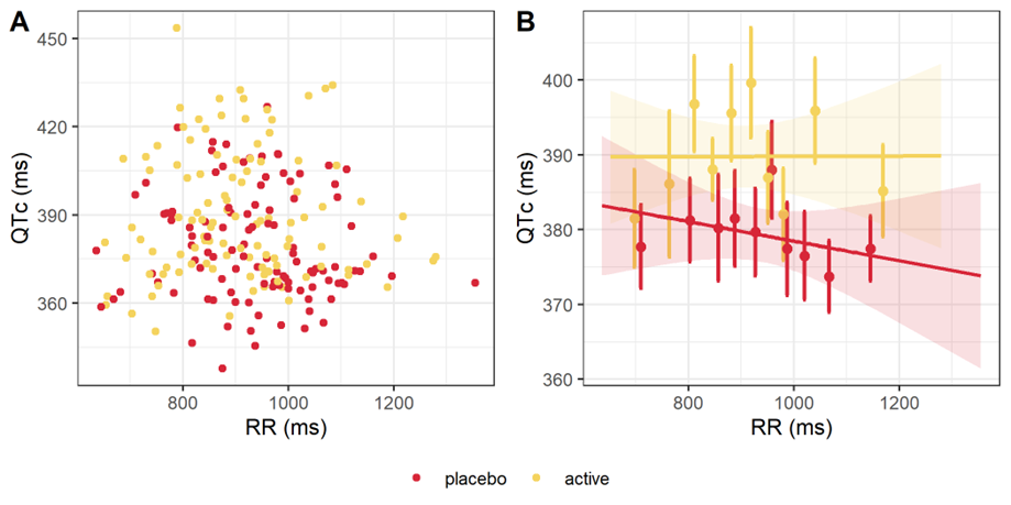
Assumption 2: QTc interval is independent of HR

After heart-rate corrected, QTc is expected to be independent from the heart rate (HR) and from its inverse, the RR interval. A scatter plot of QTc interval duration vs RR interval duration, stratified by treatment, is provided below. The linear regression for the active and placebo groups are shown in panel B. The slopes are not significantly different from 0, with p-values being respectively 0.988 and 0.368. Thus, the QTc interval is independent from RR and from HR.

QTc interval duration vs RR, overall (A) and by treatment (B).

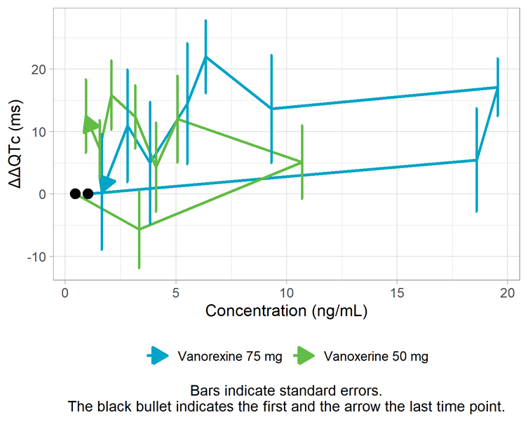
Assumption 3: No time delay between drug concentrations and ΔQTc

The assumption of a direct effect, i.e. an immediate change in ΔΔQTc following a change in concentration, is assessed visually below. With a direct effect, the effect increases and decreases with concentration on the same path. In the figure below, we observe a counterclockwise pattern which suggests the presence of hysteresis, i.e. a delayed effect. To investigate this assumption further, models with a delay will be explored in the next section “Alternative models”.

Mean ΔΔQTc per time point vs concentration

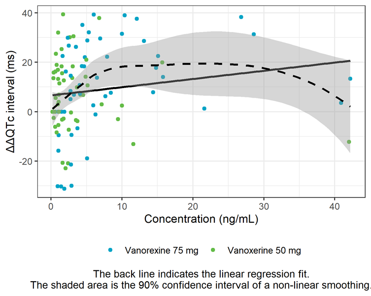
Assumption 4: Linear C-QTc relationship

The linearity assumption between exposure and ΔΔQTc is assessed by a concentration-ΔΔQTc plot with linear regression and LOESS smoother. The shape of the LOESS smoother suggests that the relationship is not linear at high doses and that an Emax model might describe the data better. This will also be investigated further in the next section.

ΔΔQTc vs concentration

Alternative models fitting

In the previous section, we have seen that the assumptions of no delay and linear relationship might not hold for the vanoxerine dataset. To explore this further, alternatives to the direct-effect linear model can be used.

It is possible to investigate other relationship shapes between drug concentration and ΔΔQTc (or ΔQTc) such as Emax, Emax with Hill coefficient, or log-linear. These models can be compared based on goodness of fit metrics such as the BICc. Furthermore, it is possible to assess if the introduction of a delay between the drug concentration and its effect on ΔΔQTc (or ΔQTc), via an effect compartment, improves the BICc. These alternative models are available in the library of models provided with the R functions.

To run all models present in the library, the function generateAllQTcProjects() can be used:

generateAllQTcProjects(dataSet="Vanoxerine_formatted.csv", 
                       IDname="SUBJID", TIMEname="TIME", TRTname="TRT", CONCname="CONC", 
                       placeboName = "Placebo", 
                       modelFolder="../_mlxQTcTools/models/ddQTcModels", 
                       projectFolder="./mlx_runs", 
                       isddQTC = TRUE, 
                       bRun = TRUE)

The arguments are similar to those of the generateQTcProject() function except that a modelFolder (containing the library models) and a projectFolder (containing the generated Monolix runs) argument are given.

The following output is generated in the console to follow the run progression and models tested:

Created project ./mlx_runs/ddQTc_Emax.mlxtran. Running project... Done.
Created project ./mlx_runs/ddQTc_Emax_effectComp.mlxtran. Running project... Done.
Created project ./mlx_runs/ddQTc_EmaxSigma.mlxtran. Running project... Done.
Created project ./mlx_runs/ddQTc_EmaxSigma_effectComp.mlxtran. Running project... Done.
Created project ./mlx_runs/ddQTc_Linear.mlxtran. Running project... Done.
Created project ./mlx_runs/ddQTc_Linear_effectComp.mlxtran. Running project... Done.
Created project ./mlx_runs/ddQTc_LogLinear.mlxtran. Running project... Done.
Created project ./mlx_runs/ddQTc_LogLinear_effectComp.mlxtran. Running project... Done.

To compare the results of the different models, a new report can be generated, which will provide comparison tables. The report is generated similarly to the first time. The only new argument is thresBICc to choose the threshold BICc value which will serve for the run comparison.

quarto_render(input = "../_mlxQTcTools/QTc_quarto_allModels.qmd", 
              output_file = "Vanoxerine_ddQTc_report_allModels.docx",
              execute_params = list(folderName = "../Example_Vanoxerine/mlx_runs",   # give relative path from quarto template (.qmd) to folder containing runs
                                    compoundName = "Vanoxerine",
                                    CONCcolumn = "CONC", 
                                    TRTcolumn = "TRT",
                                    bHasPlacebo = T,
                                    placeboName = "Placebo", 
                                    studyType = "ddQTc",
                                    concentrationUnit = "ng/mL",
                                    nBins = 10,
                                    orderTRT = c("Placebo","Vanoxerine 50 mg", "Vanorexine 75 mg"),
                                    thresBICc = 0))

In the generated report, the presence of a delay is assessed by comparing the goodness of fit (via the BICc) of the standard linear model and a linear model with an effect compartment to introduce a delay. The table below shows that the model with effect compartment is 17 points better with a delay estimated to be 2.3 hours.

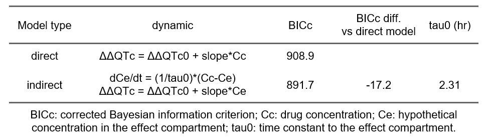
Thus, there is evidence of a delay between the drug concentration and its effect on ΔΔQTc. A delay might be caused by an active metabolite that exerts an effect on QTc such that the time delay between parent concentration and effect change actually describes the metabolism from parent drug to metabolite with the effect originating from the metabolite. In absence of knowledge or data on a possible metabolite, the delay can be described by an effect-compartment model (also called indirect model) for the observed drug concentration, as shown above.

In case of a delay, the time of maximum concentration may be substantially different from the time of maximum effect. The ΔΔQTc confidence interval cannot be derived using the usual formula anymore, where a range of Cc value is used to obtain the corresponding ΔΔQTc values. Indeed, the effect will not solely depend on the current concentration anymore but on the entire past profile of the drug concentration, as shown by the use of the time-derivative in the model. In order to obtain a ΔΔQTc confidence interval in case of a delay, it is necessary to develop a population PK/QTc model, that models not only the effect of concentration on QTc, but also the shape of the concentration over time. This is shown in the next section.

Even though a population PK/QTc model will be needed, we can nevertheless check the results of the alteratives models with different C-QTc relationship shapes:

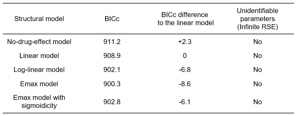
The comparison of the BICc goodness of fit metric indicates that an Emax model captures the data better (improvement of 8.6 points of BICc compared to the linear model). This is consistent with our observations based on the exploratory data analysis, and will guide the development of the population PK/QTc model.

Conclusion

The exploratory data analysis and the fitting of several alternatives to the pre-specified linear model have shown that the assumptions required to apply the linear model are not fulfilled. In particular, there a delay in the effect of the drug concentration on QTc.

In such a case, the ΔΔQTc confidence interval cannot be derived using the usual formula anymore, where a range of Cc value is used to obtain the corresponding ΔΔQTc values. In order to obtain a ΔΔQTc confidence interval in case of a delay, it is necessary to develop a population PK/QTc model, that models not only the effect of concentration on QTc, but also the shape of the concentration over time. This step cannot be done directly with the conc-QTc R package and is shown in a dedicated case study.

Read PK-QTc modeling case study