Conc-QTc modeling and implementation

Conc-QTc Modeling

Pre-specified linear model

The Garnett et al. White Paper suggests to use a linear model with concentration effect, treatment effect, time effect and centered baseline effect:

with i the individual, j the treatment and k the time. The ϴ parameters represent fixed effects and the η terms indicate random effects. It is assumed the random effects are normally distributed with mean 0 and an unstructured covariance matrix. The residual error are normally distributed with mean 0 and a constant variance.

Variations to the pre-specified model

Specific situations require adaptations of the pre-specified model, as listed in Table 4 of Garnett et al.

ΔΔQTc as dependent variable

In crossover studies where each individual receives both placebo and active treatment, it is possible to compute ΔΔQTc for each individual by subtracting the ΔQTc for placebo from the ΔQTcF for each treatment arm. In this case, ΔΔQTc can be modeled directly, leading to a simpler model. With the intercept (ϴ_0,pop+η_0,i) and time point terms, ϴ_3,T1*I_(TIME=T1) + ϴ_3,T2*I_(TIME=T2) + ..., being identical for active and placebo treatment, these terms cancel out. The parameter ϴ₁ denoting the treatment effect for ΔQTc becomes the intercept for ΔΔQTc (without random effects). A new covariate appears, the difference between centered baselines of the treatment and the placebo group.

The model reads:

with

No placebo data

If by design or ethical reasons a concurrent placebo arm was not included, it is not possible to estimate the ϴ₁ term associated to the placebo vs active treatment. The Garnett et al white paper also suggests to remove the ϴ₃ term associated to the time effect. When time-matched baseline record are used, diurnal variations are already corrected for and the ϴ₃ term is indeed not needed (see next section). However, when datasets without placebo data use predose baselines, Orihashi et al have shown that including categorical time effects in the model leads to less biased estimates and better controlled false negative rates.

The model thus reads:

Time-matched baseline

Time-matched baseline adjustments use the corresponding predose QTc measurements collected prior to drug administration on Day -1. A time-matched baseline adjustment may be used when placebo data are not available, in order to minimize the effect of diurnal variation in QTc. In case of time-matched baseline, diurnal variations are already corrected for and the ϴ₃ term is not needed.

The model reads:

Note that if there is no placebo data, the ϴ₁ term also drops out (see section above).

Data over multiple days

If QTc measurements are collected over multiple days, the TIME parameter can be reduced to time after dose on same day and DAY is included in model as an additional factor.

The model reads:

Non-linear concentration effect

If exploratory plots indicate a non-linear effect of the concentration on ΔQTc, alternative models can be used. Typical non-linear models are Emax, Emax with sigmoidicity (Hill) and loglinear relationships.

Emax model:

Emax with sigmoidicity (Hill equation):

Loglinear model:

Implementation in Monolix

Monolix is a tool for parameter estimation and model diagnostic for linear and non-linear mixed-effects models. It can thus be used to implement and use the models presented above. The implementation in Monolix requires to slightly reorganize the model into two distinct pieces (still corresponding to the same final equation).

The implementation of the model will be done automatically in the R package. This section is for information purpose but does not need to be applied to the user himself.

Separation into structural and statistical model

In a pharmacometric framework, the pre-specified linear model can be rewritten as a structural model which described the drug effect on ΔQTc:

and a statistical model, which describes the interindividual variability and covariate effects:

This formulation allows for an easy extension to non-linear relationships between ΔQTc and the concentration, by defining alternative structural models. The implementation of the other variations to the pre-specified model are easily implemented by including less or different covariates.

For ϴ_0,i, we would like to consider random effects varying from individual to individual (η_0,i) and covariates which varies from period to period (TRT, BLQTc_cent) or from time point to time point (TIME). Due to a limitation in Monolix, this forces us to separate the fixed effects and the random effects into two different terms of the structural model.

The structural model we will use is thus:

and the individual model is:

The term ϴ_0,i now contains only fixed effects: the intercept ϴ_0,pop and the covariate effects ϴ_1, ϴ_3,k, and ϴ₄. The term η_0,i represents the random effects for the intercept. We will fix its typical value η_0,pop to zero such that the term contains only random effects. The slope remains as before with a random and a fixed component.

Structural model in mlxtran language

In Monolix, the structural model is defined via a txt file using mlxtran language. The concentration is passed as a regressor (to be read directly from the dataset) and its effect is defined in the structural model.

The content of the mlxtran file for the linear model for ΔQTc is:

[LONGITUDINAL]
input = {Cc, dQTc0, eta_dQTc0, slope}
Cc = {use=regressor}

EQUATION:
dQTc = dQTc0 + eta_dQTc0 + slope*Cc

OUTPUT:
output = dQTc

with dQTc0 corresponding to the ϴ_0,i individual parameter (with fixed effect and covariate effects), eta_dQTc0 corresponding to η_0,i (random effects only) and slope corresponding to the ϴ_2,i individual parameter (with fixed effect and random effects).

Statistical model in the GUI

The statistical model is defined in the graphical user interface (or via the lixoftConnectors).

For ΔQTc, we will set:

• dQTc0: normal distribution to ensure that covariate are added linearly into the model, no random effects, and covariates TRT (categorical), TIME (categorical) and BLcent (continuous),

• eta_dQTc: normal distribution, with random effects, and typical population value fixed to zero,

• slope: normal distribution with random effects.

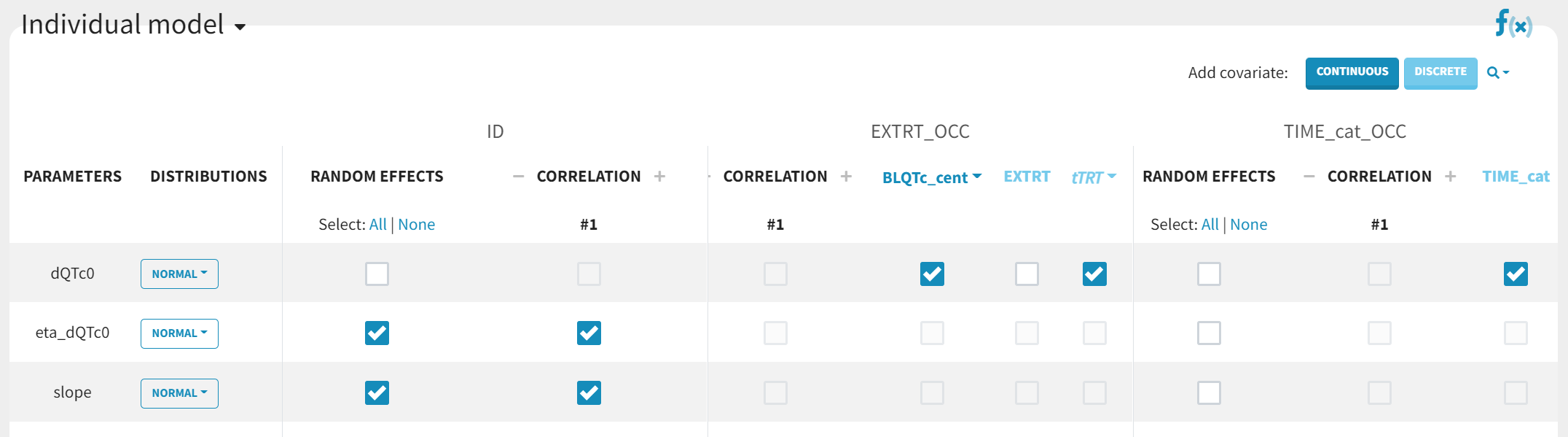
The equations corresponding to this setup can be displayed with the “equation” icon:

The typical value for the eta_dQTc0 parameter is fixed to zero in the Initial Estimates tab.

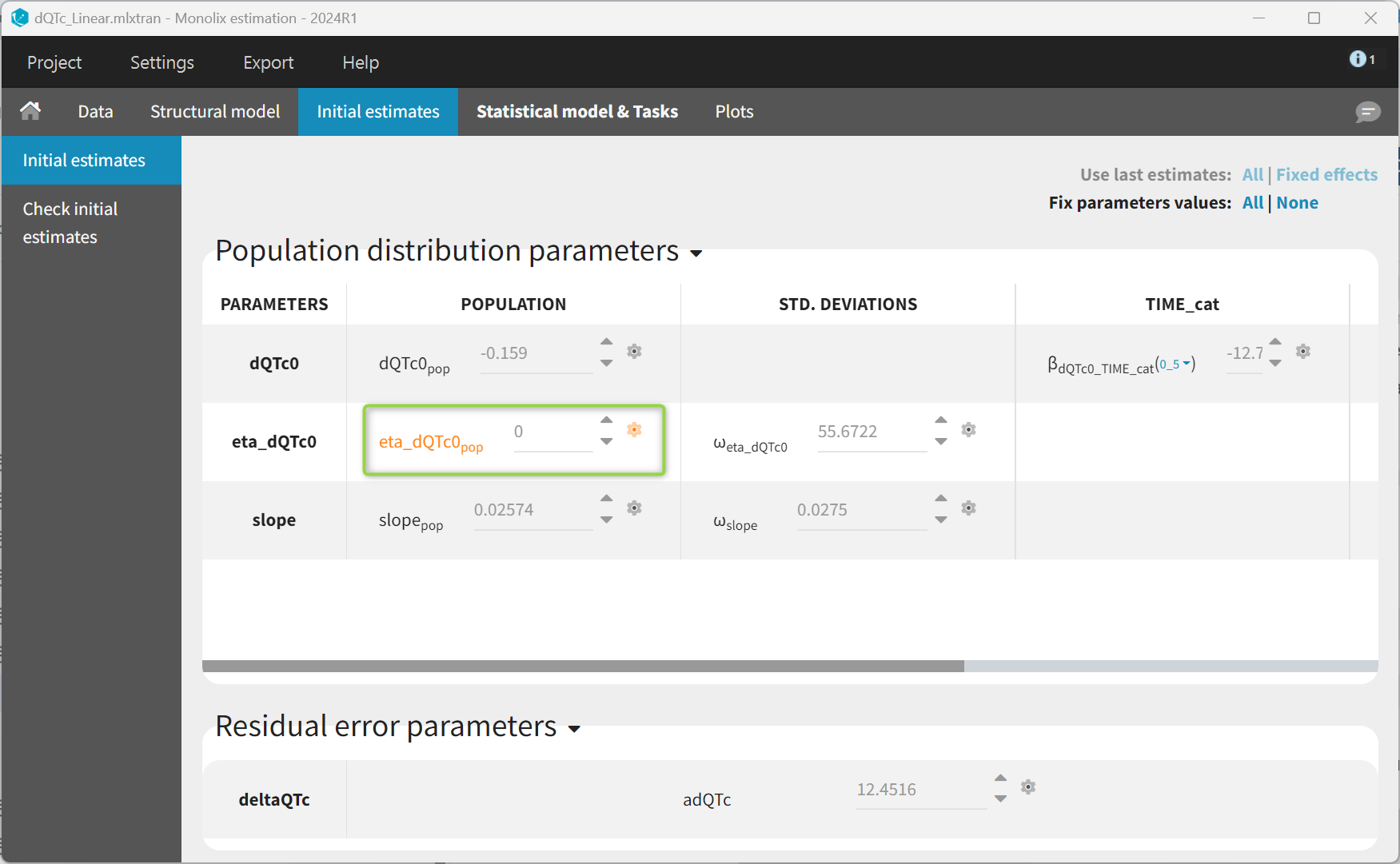
We consider correlations between the random effects (which corresponds to an unstructured covariance structure) and a constant residual error model, as suggested in Garnett et al.

Parameter estimation

Running the “population parameters” task will estimate the model parameters using the SAEM algorithm. The standard errors task will estimation the Fisher information matrix (FIM), the variance-covariance matrix of the estimates and the corresponding relative standard errors (RSE). They represent the uncertainty of the estimated parameters and will be used in the next section to compute the confidence interval.

Model-derived ΔΔQTc at concentration(s) of interest

Derivation of the ΔΔQTc equation

The conc-ΔQTc model is used to compute the ΔΔQTc at concentrations of interest. The concentrations of interest are typically concentrations at the therapeutic dose in a patient population
taking into account possible concentration increase due to drug interactions, impaired hepatic or renal function, and polymorphisms in CYP enzymes. The concentrations of interest should be inside the range of observed concentrations used to generate the model, such that the model is used for interpolation but not extrapolation.

The PD metric of interest is ΔΔQTc, the change from baseline QTc adjusted for placebo. It is calculated as the difference between the model-derived ΔQTc at the concentrations of interest and model-derived ΔQTc for placebo with concentration = 0.

Because the intercept (ϴ_0,pop+η_0,i) and time point terms, ϴ_3,T1*I_(TIME=T1) + ϴ_3,T2*I_(TIME=T2) + ..., are identical for the two terms, they cancel out. The parameter ϴ₁ (treatment effect) which is present only for the first term remains. The BLQTc_cent is assumed to be null on average and is ignored. The random effects for the slope η_2,i are also averaged by the mean. We thus obtain:

with Est denoting the estimate of the true value.

To calculate the confidence interval, an analytical formula can be derived when the linear model is used (see Garnett et al.), based on the standard errors of the estimates. However, this formula cannot be generalized when non-linear models are used. An alternative would be to use non-parametric bootstrap, but this would require many runs. In Monolix, we can use the variance-covariance matrix of the estimates (from which the standard errors are derived) to sample sets of (ϴ₁, ϴ₂) parameters which capture their uncertainty, instead of using bootstrap replicates. Each set is used to generate a ΔΔQTc prediction and the 90% confidence interval is calculated based on these predictions, as described in Garnett. et al.

The resulting plot overlays the ΔΔQTc model prediction (black line), its 90% prediction interval capturing the uncertainty (blue band), the 10 ms increase in ΔΔQTc threshold (dashed line) and the upper limit of the prediction interval at the concentration of interest (blue arrow).

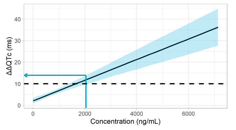
Implementation in Simulx

In order to reuse directly the developed model for ΔQTc, we will calculate the ΔΔQTc as the difference between the model-derived ΔQTc at the concentrations of interest and model-derived ΔQTc for placebo with concentration = 0.

To perform the model prediction, the Monolix project is exported to Simulx. We will consider two simulation groups, one for the active treatment and one for the placebo.

The simulation setup is the following:

• parameters: the random effects are ignored and the fixed effects are sampled from the uncertainty distribution. This is done by selecting the element “mlx_TypicalUncertainLin”.

• covariates: the TRT covariates is set to 1 for the active group and 0 for the placebo. The values for the BLQTc_cent and TIME covariates are set to 0 and will anyway cancel out.

• concentration: a fine grid of concentrations of interest is defined, via the regressor element. For the placebo group, the concentration is set to zero.

• replicates: 500 replicates are used, each corresponding to a different set of population parameters sampled from the covariance matrix of the estimates (uncertainty distribution)

• group size: for each replicate, a single simulation is done (as the random effects are ignored, all simulations would be identical)

Outside of Simulx, we compute ΔΔQTc as the difference between the predictions of the two groups, for each replicates. The 5th, median and 95th percentiles over replicates is finally computed.

This procedure for both linear and non-linear models and any included covariates.