This example shows how to perform Bayesian individual dynamic predictions. Using an existing population PK model with estimated population parameters as prior, samples from the conditional distribution (i.e posterior) are obtained for each individual of a new dataset, to capture the uncertainty of the individual parameters given the observations.
Step 1: sampling from the conditional distribution
We will use the demo Theophylline project as an example, using loadProject(). If population parameters have not been estimated yet, the task must be run with runPopulationParameterEstimation().
library("lixoftConnectors")
library(dplyr)
library(ggplot2)
initializeLixoftConnectors(software = "monolix", force=T)
# load demo project
project <- paste0(getDemoPath(), "/1.creating_and_using_models/1.1.libraries_of_models/theophylline_project.mlxtran")
loadProject(projectFile = project)
# run parameter estimation (if needed)
runPopulationParameterEstimation()
In order to use the estimated population parameters as a prior (and not re-estimate them based on the new dataset), we update the initial values based on the previous estimates with setInitialEstimatesToLastEstimates() and then fix them using setPopulationParameterInformation().
setInitialEstimatesToLastEstimates()
popparams <- getPopulationParameterInformation()
popparams$method <- "FIXED"
setPopulationParameterInformation(popparams)
The next step is to load the new dataset containing the individuals for which we want to perform the Bayesian prediction. In this example, we reuse the original dataset but truncate the time at 10h, to investigate the impact of a shorter trial duration. The observations from this new dataset are also saved in a R object which will be used later to overlay the observations of the prediction plot.
baseDataset <- read.table(getData()$dataFile, header=T)
filteredDataset <- baseDataset[baseDataset$TIME<10,]
write.csv(filteredDataset, "filteredDataset.csv", row.names = F, quote=F)
setData("filteredDataset.csv", getData()$headerTypes, getData()$observationTypes)
# save for plotting later
obsData <- getObservationInformation()$CONC
By default only a few samples from the conditional distribution are saved. In order to obtain a nice prediction interval, we will save 200 samples. This is done by using nbsimulatedparameters=200 in setConditionalDistributionSamplingSettings(). The samples are taken uniformly over an interval of nbminiterations iterations. Given that two samples next to each other have a risk to be identical, we usually set nbminiterations = 3 x nbsimulatedparameters to use one sample every 3 iterations. When nbminiterations is large, the convergence criteria are harder to achieve. To avoid running for very long, we can give a max number of iterations with enableMaxIterations=T and nbMaxIterations=1200. The call is done in two steps due avoid being temporarily in a situation where nbminiterations>nbMaxIterations (which is forbidden).
setConditionalDistributionSamplingSettings(enableMaxIterations=T, nbMaxIterations=1200)
setConditionalDistributionSamplingSettings(nbminiterations=600, nbsimulatedparameters=200)
The project can then be saved (to avoid overwriting the original run) and run. Even if the population parameters are fixed, the task Pop param must be run before running the conditional distribution task. We then retrieve the samples from the conditional distribution with getSimulatedIndividualParameters().
saveProject("bayesian_forecasting.mlxtran")
runPopulationParameterEstimation() # mandatory before other tasks, but nb of iterations is null as all parameters are fixed
runConditionalDistributionSampling() # this is sampling from the posterior distribution for each individual
# retrieve the samples from the conditional distribution
samplesCondDistrib <- getSimulatedIndividualParameters()
The samplesCondDistrib contains one line per id and per sample (column rep).
> head(samplesCondDistrib)
  rep id        ka         V         Cl
1   1  1 1.9582949 0.3939064 0.02888324
2   1  2 2.1925275 0.4230115 0.05076061
3   1  3 1.6761378 0.4503078 0.04192262
4   1  4 1.2335670 0.5261603 0.03801980
5   1  5 1.5879271 0.5561964 0.04986806
6   1  6 0.9479706 0.4571833 0.04743354
Step 2: simulation using the samples for each individual
To simulate the prediction corresponding to the 200 samples of each individual, we will use Simulx. For this, we will define an Individual parameter element containing the samples. However, this type of element can have an “id” column but not both an “id” and a “rep” column. We will thus work replicate per replicate. Note that it would not be possible to merge the id and rep column into a single one, because then the ids would be renamed and the matching to the id column of the treatment or regressor elements would be broken.
The first step is to export from Monolix to Simulx.
exportProject(settings=list(targetSoftware="simulx"), force=T)
By default, a simulation is already setup with the same number of individuals (size), treatment (mlx_Adm1), covariates (if applicable) and regressors (if applicable) as in the dataset used in the Monolix project. The population parameters are used by default, and we will change this later to use the sampled individual parameters.
> printSimulationSetup()
$simulationGroups
           simulationGroup1
size                     12
parameters          mlx_Pop
treatments         mlx_Adm1
outputs            mlx_CONC
The simulation is performed into a for loop going over the replicates (i.e samples). Within each iteration of the loop, all individuals are simulated with sample i. To define the individual parameter element, we need to provide a csv file. We thus filter the samplesCondDistribto keep only replicate i and save this as a csv file. The individual parameters element is defined in Simulx using defineIndividualElement(). In addition, we can define an output element to control de time grid of the prediction using defineOutputElement(). In this example, we use the smooth (without residual error) model output called Cc. The two created element, called samplesCondDistrib and outCc are applied to the simulation using setGroupElement(group = "simulationGroup1", elements = c("samplesCondDistrib","outCc")). Note that simulationGroup1 is the default name, as visible above when using printSimulationSetup(). To ensure that the ids of the individual parameter and other elements (here treatment mainly) are correctly mapped together, we use setSharedIds(sharedIds = c("output", "treatment", "regressor", "individual")). The simulation is then run with runSimulation() and the results are retrieved with getSimulationResults(). The replicate information is added to the result data.frame and the results for all replicates are merged.
sims <- NULL
for(i in unique(samplesCondDistrib$rep)){
  cat(paste0("Replicate ", i, " out of ", length(unique(samplesCondDistrib$rep)), "\r"))
  # the samples are filtered for the current replicate and the rep column is removed
  samplesCondDistrib_repI <- samplesCondDistrib[samplesCondDistrib$rep==i,c(-1)]
  # save as a csv file (it is not possible to give a data.frame as input to defineIndividualElement)
  write.csv(samplesCondDistrib_repI, "samples_repI.csv", row.names = F, quote=F)
  # define an element from an external file containing the samples from the conditional distribution
  defineIndividualElement(name="samplesCondDistrib", element="samples_repI.csv")
  # define output time grid
  defineOutputElement(name="outCc", list(data = data.frame(start = 0, interval = 0.1, final = 24), output = "Cc"))
  # use the defined element for the simulation
  setGroupElement(group = "simulationGroup1", elements = c("samplesCondDistrib","outCc"))
  # make sure the ids of each element are correctly mapped together
  setSharedIds(sharedIds = c("output", "treatment", "regressor", "individual"))
  # run the simulation
  runSimulation()
  # retrieve the results
  sim_repI <- getSimulationResults()$res$Cc
  # add replicate information
  sim_repI$rep <- i
  # merge all replicates
  sims <- rbind(sims, sim_repI)
}
Step 3: plotting
To plot the prediction interval of each individual, we calculate the 5th, median and 95th percentile over the replicates for each individual and each time point. The prediction interval is then plotted with ggplot, stratified by id and the data is overlayed.
prctle <- sims %>% group_by(original_id,time) %>%
  summarise(P05=quantile(Cc,0.05),
            P50=quantile(Cc,0.5),
            P95=quantile(Cc,0.95)) %>%
  ungroup() %>%
  rename(id=original_id)


ggplot(prctle) + geom_ribbon(aes(x=time,ymin=P05,ymax=P95), fill="#ff793f", alpha=0.5) +
  geom_line(aes(x=time,y=P50), color="#ff793f") +
  geom_point(data=obsData, aes(x=time,y=CONC)) +
  facet_wrap(.~id)+
  ylab("Conentration")+
  xlab('Time (hours)')+theme_bw()
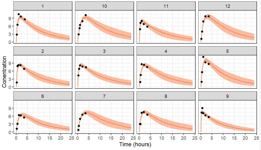
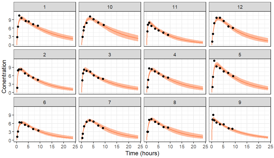
The resulting plot is the following with data truncated at 10 hours.
If the data is truncated at 4 hours instead, we have less data and thus a higher uncertainty in the individual parameters. This leads to wider prediction intervals. For individuals which have no data information the elimination rate, the prediction of the elimination phase is mostly based on the population parameters which were used as a prior.