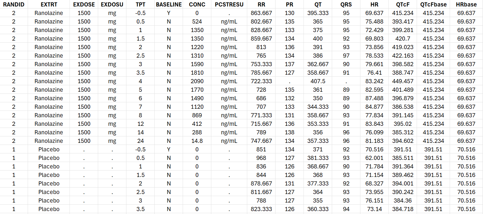
Original data
In this example, we use a modified version of the data presented in Johannesen et al. and available for download. The original data is a 5-way crossover study in 22 healthy subjects. PK and QT data were collected at 16 matching time points over 24 h after dose administration.
For this example we will use only the placebo and ranolazine periods. In addition, we rename the IDs to create a unique ID for each id and period combination, to mimic a parallel design where each individual has a single period and has received either placebo or ranolazine.
The HR, QTcF, QTcFbase and HRbase columns were added manually to show an example of the usage of process_QTcData()when these columns are already present in the dataset.
The csv file we will start from contains the following columns:
Data processing
In order to use the provided R functions, the R script mlxQTcTools.R must be sourced. In addition, a monolixSuite installation must be available and the lixoftConnectors R package installed. In order to indicate the location of the MonolixSuite installation, the functioninitQTc(path=...) is used.
source('../_mlxQTcTools/mlxQTcTools.R')
initQTc(path="C:/Program Files/Lixoft/MonolixSuite2024R1")
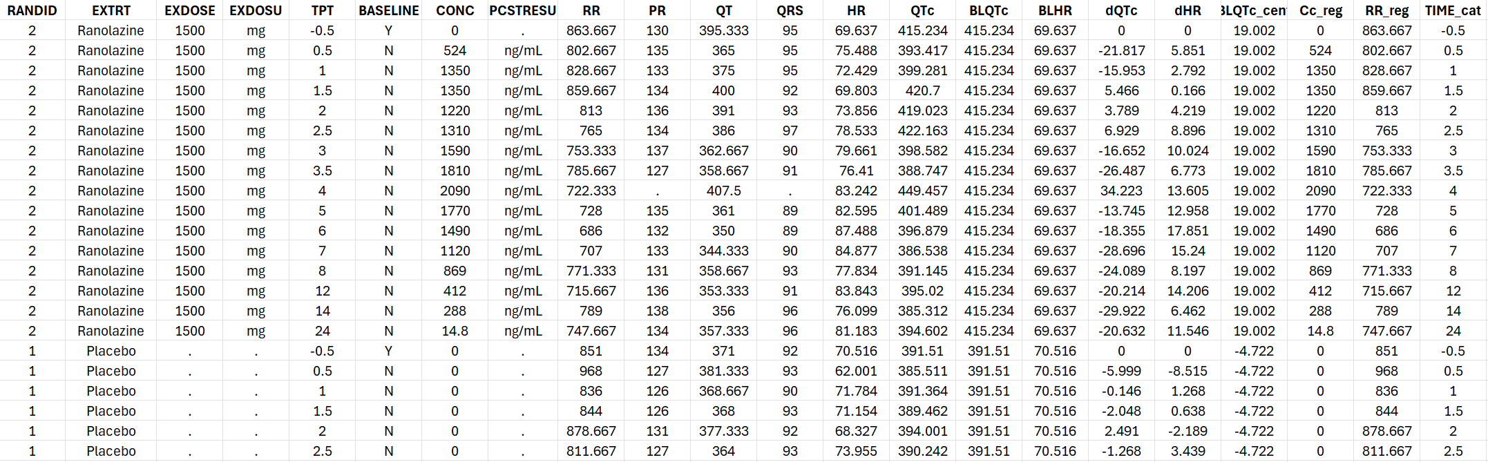
In the initial dataset, the QTc has already been calculated, the triplicates have been averaged and the baseline QTc and HR columns are present. In order to perform a concentration-QTc analysis, the steps that remain to be applied are:
-
calculate the baseline-corrected QTc, i.e ΔQTc.
-
for exploratory data visualization purpose, calculate the ΔHR
Covariates and regressor variables which will appear in the conc-QTc model are also added as additional columns:
-
the centered QTc baseline
-
time as categorical factor
-
concentration and RR interval duration
The steps can be performed using the function process_QTcData():
process_QTcData(data="Ranolazine_data_parallel.csv",
                QTname = "QT", RRname = "RR", HRname = "HR",
                CONCname = "CONC", TRTname = "EXTRT", IDname = "RANDID", TIMEname = "TPT",
                bComputeBaseline = FALSE, BLQTCname = "QTcFbase", BLHRname = "HRbase",
                bComputeQTc = FALSE, QTCname="QTcF",
                outName = "Ranolazine_formatted.csv", silent=F)
The column containing the QT, RR, HR, drug concentration, treatment (placebo or drug), subject id and time are indicated using the arguments QTname, RRname, HRname, CONCname, TRTname, IDname, TIMEname. Note that the values present in the TRTname column will be used as plot labels for the report. In this example, the column contains “Placebo” and “Ranolazine”.
Given that the QTc column (heart rate-corrected QT) is already present in the dataset, it does not need to be computed and we set bComputeQTc = FALSE. The name of the QTc column is indicated using the QTCname argument.
The QTc baseline and HR baseline columns are also already present in the dataset. We thus use bComputeBaseline = FALSE and indicating the arguments BLQTCname (QTc baseline) and BLHRname.
The name of the output file is given via the outName argument.
Running the function on the Ranolazine example generates the following console output:
Info: The following treatment groups have been found: Ranolazine, Placebo
Info: The dQTc and dHR columns have been calculated as dQTc=QTc-BLQTc and dHR=HR-BLHR.
Info: The BLQTc_cent column has been calculated as BLQTc_cent=BLQTc-mean(BLQTc).
Info: Some individuals have no placebo data. ddQTc will not be calculated.
Info: The Cc_reg (concentration as regressor), RR_reg (RR as regressor) and TIME_cat (TIME as categorical covariate) columns have been added.
 ==> Created new dataset Ranolazine_formatted.csv.
The Info lines give details about the data processing steps. The Warning lines draw attention on unusual situations such as missing concentration on lines not belonging to the placebo group. The console output can be avoided using silent=T.
Note that ΔΔQTc could not be computed because each individual has received either placebo or the drug but not both. The QTcF, QTcFbase, HRbase column which were already present have been renamed to follow the standard name required for the generateAllQTcProjects()function.
The generated formatted dataset is the following. It contain all columns needed to create a Monolix project for conc-QTc analysis as well as creating the usual exploratory data analysis plots.
Model fitting
The next step is to generate and run Monolix projects to estimate the parameters of the concentration-ΔQTc models. Both linear and non-linear conc-QTc relationships are considered.
To generate and run the Monolix projects to run the con-QTc analysis, the function generateAllQTcProjects() is used.
generateAllQTcProjects(dataSet="Ranolazine_formatted.csv",
                   IDname="RANDID", TIMEname="TPT", TRTname="EXTRT",
                   CONCname="CONC", placeboName = "Placebo",
                   modelFolder="../_mlxQTcTools/models/dQTcModels",
                   projectFolder="./mlx_runs",
                   isddQTC = FALSE,
                   bRun = TRUE)
The user should provide the formatted dataset in the argument dataSet, as well as the name of the columns containing the subject id in IDname, time in TIMEname, treatment groups in TRTname, concentration in CONCname. The other columns (e.g QT, QTc, HR, etc) must have predefined headers and do not need to be specified.
The category of the treatment group column representing placebo can be indicated using placeboName = "Placebo". If this argument is omitted, the function will search for the string “placebo” among the categories present in the TRT column.
The folder containing the structural models to be used to generate the monolix runs are given in the argument modelFolder. The R package contains a pre-written library of models with linear, Emax, Emax with sigmoidicity and loglinear conc-QTc relationship. User-defined models can be added to this folder is needed. In folder in which the runs are generated is the projectFolder argument.
Whether conc-ΔΔQTc or conc-ΔQTc should be run is indicated using isddQTC = T or F. To run the projects after having created them, use bRun = T.
When running the function, the console output indicates the generated runs, the implemented models and the progress of the parameter estimation:
[INFO] The specified directory 'projectFolder' did not already exist and was created C:/Users/geral/Workspace/R_packages/conc_QTc/Example_Ranolazine/mlx_runs
Created project ./mlx_runs/dQTc_Emax.mlxtran with model:
     dQTc = (theta0 + eta0) + theta1 * TRT + theta3 * TIME_cat + theta4 * BLQTc_cent + (theta2 + eta2) * Conc/(Conc + theta5)
     Running project... Done.
Created project ./mlx_runs/dQTc_EmaxSigma.mlxtran with model:
     dQTc = (theta0 + eta0) + theta1 * TRT + theta3 * TIME_cat + theta4 * BLQTc_cent + (theta2 + eta2) * Conc^theta6/(Conc^theta6 + theta5^theta6)
     Running project... Done.
Created project ./mlx_runs/dQTc_Linear.mlxtran with model:
     dQTc = (theta0 + eta0) + theta1 * TRT + theta3 * TIME_cat + theta4 * BLQTc_cent + (theta2 + eta2) * Conc
     Running project... Done.
Created project ./mlx_runs/dQTc_Linear_effectComp.mlxtran with model:
     dQTc = (theta0 + eta0) + theta1 * TRT + theta3 * TIME_cat + theta4 * BLQTc_cent + (theta2 + eta2) * Ce with dCe/dt = (Conc - Ce)/theta5
     Running project... Done.
Created project ./mlx_runs/dQTc_LogLinear.mlxtran with model:
     dQTc = (theta0 + eta0) + theta1 * TRT + theta3 * TIME_cat + theta4 * BLQTc_cent + (theta2 + eta2) * log(1 + Conc/theta5)
     Running project... Done.
The generated Monolix runs can be opened with the Monolix GUI for inspection.
Report generation
A standard report can be generated using the function quarto_render() and a Quarto template. The quarto template will read the results from generated Monolix projects and generate a report including:
-
Exploratory data analysis (data summary, QT/QTc, heart rate correction, baseline QTc, ΔQTc and concentration-time)
-
Model assumption assessments (heart-rate independence from drug concentration, QTc independence from heart rate, linearity of the concentration-QTc relationship, immediate effect of concentration change on ΔQTc change)
-
Modeling results (comparison of the different models, model fit, parameter estimates, goodness of fit)
-
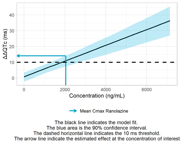
Derivation of the ΔΔQTc prediction intervals, including assessment of the 10-ms threshold
The quarto function is called in the following way:
quarto_render(input = "../_mlxQTcTools/QTc_quarto_allModels.qmd",
              output_file = "Ranolazine_dQTc_report.docx",
              execute_params = list(folderName = "../Example_Ranolazine/mlx_runs",   # give relative path from quarto template (.qmd) to folder containing runs
                                    compoundName = "Ranolazine",
                                    CONCcolumn = "CONC",
                                    TRTcolumn = "EXTRT",
                                    bHasPlacebo = TRUE,
                                    placeboName = "Placebo",
                                    studyType = "dQTc",
                                    concentrationUnit = "ng/mL",
                                    nBins = 10,
                                    thresBICc = 0))
The input is the quarto template. A standard quarto template is provided in the package but it can also be adjusted to the users need. The output_file indicates the name of the generated report as word document. The execute_params list the folder containing the Monolix runs in folderName, the string to be used as compound name in compoundName, the column of the formatted dataset containing the concentration in CONCcolumn, the column containing the treatment categories in TRTcolumn, the header/label to be used for the stratification column (here the TRTcolumn) in STRATname(default: “Treatment” and omitted in this example), a logical to indicate whether the dataset contains placebo data in bHasPlacebo, the placebo name in the treatment group column in placeboName, the type of study using studyType = "dQTc", the concentration unit in concentrationUnit(for plot labels), the number of bins to average the concentration in nBins, and the BICc threshold to consider that an alternative model is better than the linear model in thresBICc.
Note that the folderName must indicate the relative path from the .qmd template (not the R working directory) to the folder containing the runs.
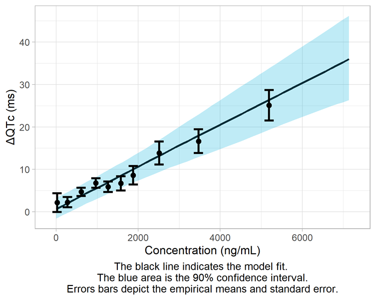
The generated report can be visualized below:

Download the generated the ΔQTc Ranolazine report (word format).
Conclusion
The conc-ΔQTc data for Ranolazine is best captured by the standard linear model from the Garnett et al white paper. The upper bound of the 90% confidence interval at the geometric mean maximum concentration is 14.1 ms and slightly exceeds the 10 ms threshold.