Observations vs predictions

Purpose

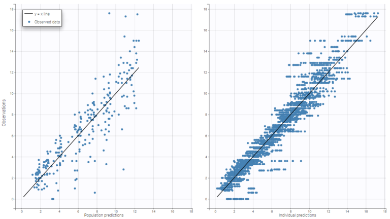
This figure displays observations () versus the corresponding predictions () computed using either the population parameters and covariate effects but random effects set to 0, or with the individual parameters. This figure is useful to detect misspecifications in the structural model. The 90% prediction interval, which depends on the residual error model, can be overlaid. Predictions that are outside of the interval are denoted as outliers. A high proportion of outliers suggest misspecifications in the model. Moreover, the  distribution of the observations should be symmetrical around the corresponding predicted values.

Population and individual predictions vs observations

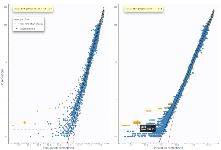
The following example corresponds to the observations and predicted concentrations for the PK of warfarin, modeled by a one-compartment model with a first-order absorption and a linear elimination. On the left, predictions are made using the population parameters while on the right they correspond to the individual parameters. More points appear with the individual predictions: for each observation point, ten predictions are displayed, corresponding to ten simulated individual parameters.

Visual guides

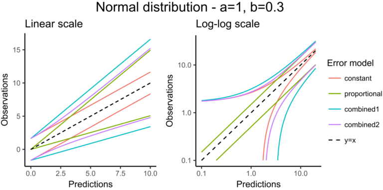
In addition to the line y = x, it is possible to display the 90% prediction interval, as well as a spline interpolation.
The 90% prediction interval represents the uncertainty of predictions due to the residual error model defined in the observation model. In the figure below, the shape of this interval can be seen for the four existing residual error models (constant, proportional, combined1, combined2) when the observation model is defined with a normal distribution:

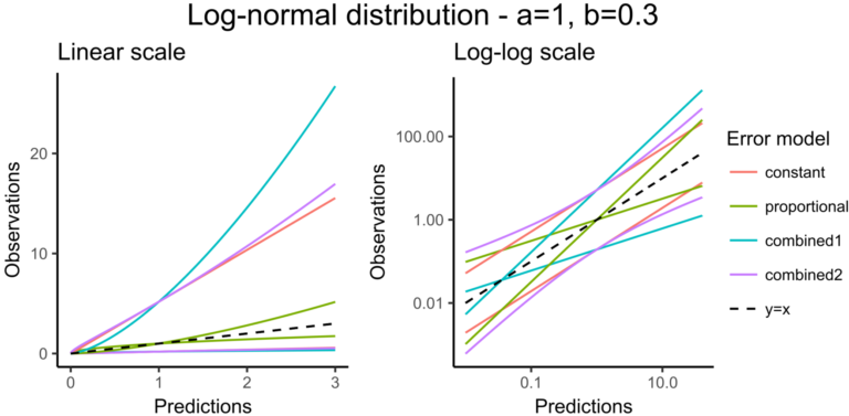
The next figure corresponds to data that follow a log-normal distribution. The combination of constant error model and log-normal distribution corresponds to an exponential error model. Error models with a proportional term can cause numerical issues with the log-normal distribution for small observations because the error becomes very small as well.

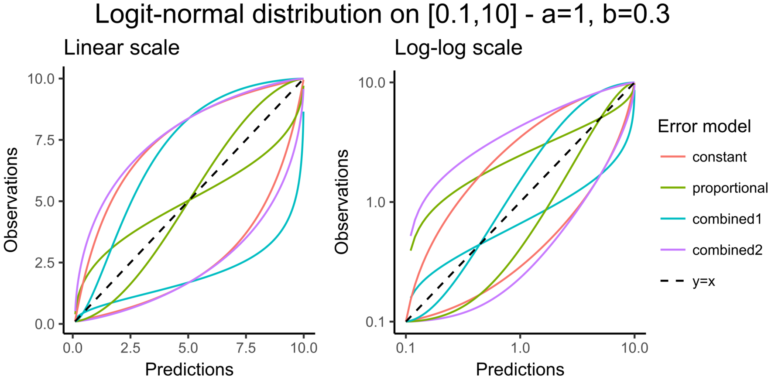
Choosing an observation model with a logit-normal distribution for the data is useful to take into account bounded data. The figure below shows the shape of the prediction intervals for the different error models associated with data that follow a logit-normal distribution in [0.1-10]:

The prediction interval for the same example as above on the PK of warfarin characterizes a residual error model that combines a constant and a proportional term:

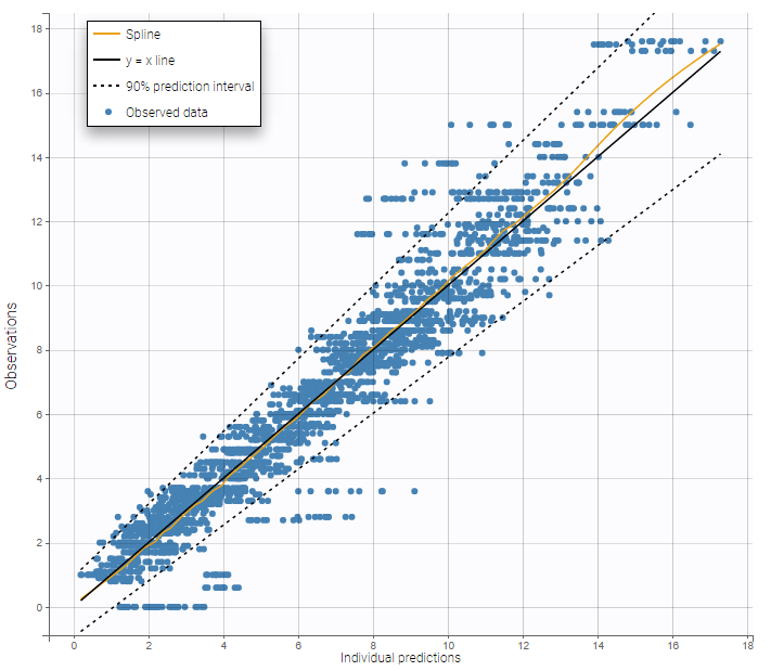
On the figure above it can be noted that several zero observations measured at low times correspond to nonzero predictions that fall outside the 90% prediction interval, and thus cannot be explained by the residual error. This could be explained by a delay between the administration and absorption of warfarin, therefore a model with a delayed absorption might fit better the data.

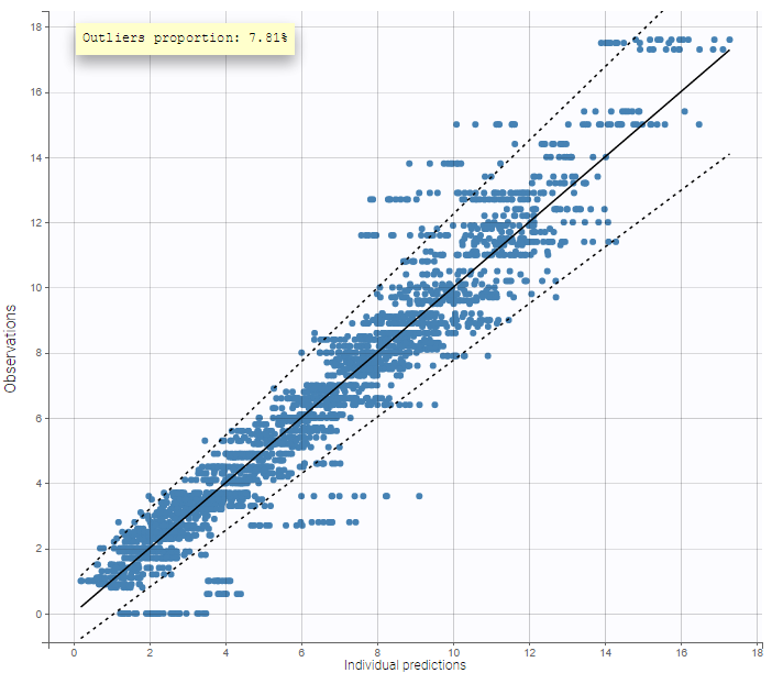
Outliers proportion

The outliers proportion can be displayed: it is the proportion of residuals outside the 90% prediction interval.

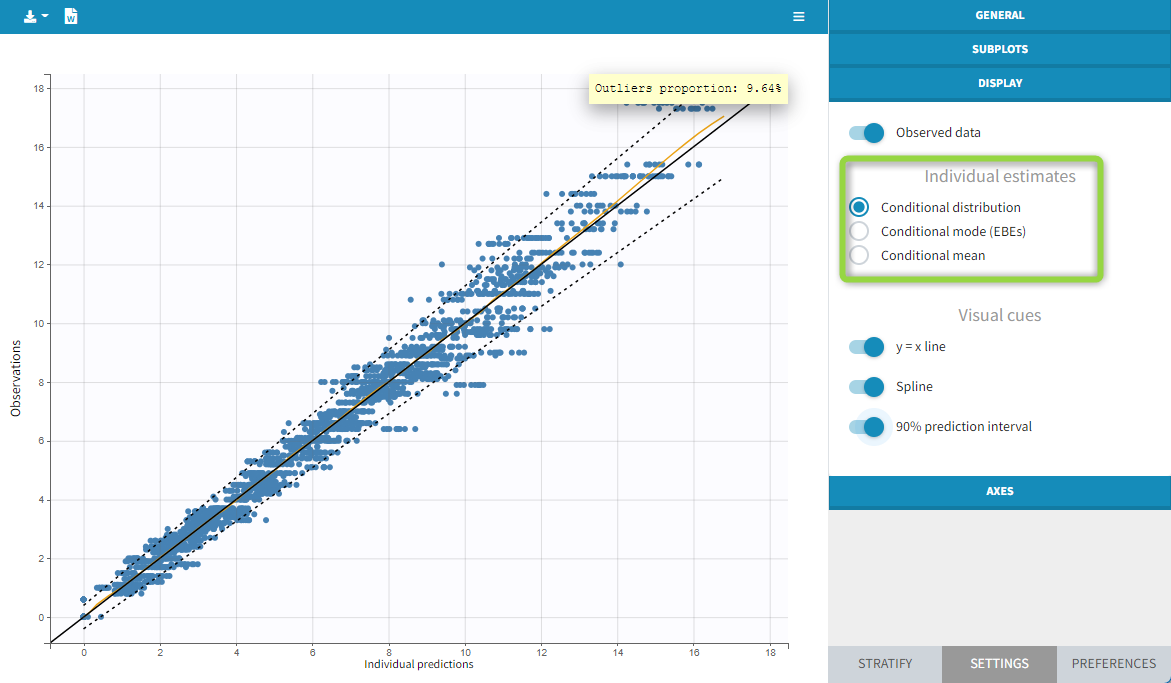
Individual estimates

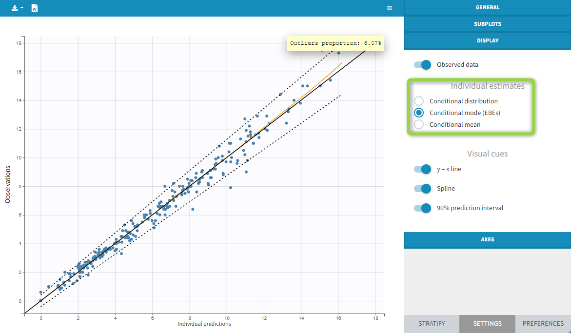
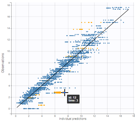
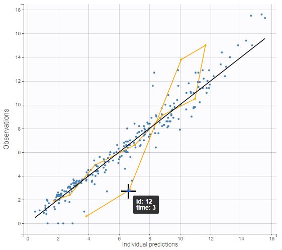
As for all diagnosis plots based on individual parameters, it is possible to choose the individual estimates that are used to compute the plot of observations vs individual predictions, among the different estimates computed during the individual parameter estimation: conditional modes (EBEs) or means of the conditional distributions, or simulated individual parameters drawn from the conditional distributions (by default). In the latter case, each observation is associated with a set of individual predictions derived from a set of individual parameters simulated from the same individual conditional distribution. On the two figures below, one can compare the plot based on simulated parameters from the conditional distribution (top) and the same plot based on conditional modes (bottom).

Highlight

As shown on the figures below, hovering on a point of observed data reveals the subject id and time corresponding to this point. All the points corresponding to this subject are highlighted in yellow. On the left, there are several predictions per observation, and the ten points corresponding to the hovered observation are indicated with a bigger diameter. On the right, there is only one prediction per observation, and all points corresponding to the same individual are linked with segments to visualize the time chronology.

Log scale

A log scale is useful to focus on low observation values. It can be set for each axis separately or both together.
A second example below displays the predicted concentrations of remifentanil, modeled by a two-compartments model with a linear elimination. In this example, the log-log scale reveals a clear misspecification of the model: the small observations are under-predicted. These observations correspond to high times: this means that the elimination is not properly captured by the two-compartment model. A three-compartment model might give better results.
that here 10 predictions are displayed for each observation, corresponding to different simulated parameters drawn from the conditional distribution during the individual parameter estimation task.

Settings

• General

  • Legend and grid : add/remove the legend or the grid. There is only one legend for both plots.

  • Outliers proportion: display/hide the proportion of points outside the 90% prediction interval.

• Subplots

  • Population prediction: add/remove the figure with the comparison between the population predictions and the observations.

  • Individual prediction: add/remove the figure with the comparison between the individual predictions and the observations.

•  Display

  • Observed data: Add/remove the points corresponding to pairs of observations and predictions.

  • BLQ data : show and put in a different color the data that are BLQ (Below the Limit of Quantification)

  • Individual estimates: select the estimates condition mean or mode, or simulated estimates from the conditional distribution (by default).

  • Visual cues: add/remove visual guidelines such as the line y = x, a spline interpolation, and the 90% prediction interval indicated with dotted lines.

By default, only the individual predictions are displayed.