Time-to-event data models

Related resources on modeling time-to-event data in Simulx:

• Time-to-event observation model: details on the different models for time-to-event data that can be used in Simulx and their syntax.

• Time-to-event model library: detailed description of the library of time-to-event models integrated within Simulx.

On the current page, we show examples of time-to-event data models from the Simulx demos, discuss the possibility to consider repeated interval-censored events as count data, and explain the format of simulated time-to-event data.

Single event

To begin with, we will consider a one-off event. Depending on the application, the length of time to this event may be called the survival time (until death, for instance), failure time (until hardware fails), and so on. In general, we simply say “time-to-event”. The random variable representing the time-to-event for subject i is typically written Ti.

Single event exactly observed or right censored

• 7.1.tte/tte_single_event.smlx (model=lib:weibull_model_singleEvent.txt)

In this Simulx demo, a Weibull TTE model for single events, taken from the TTE library, is used:

[LONGITUDINAL]
input = {Te, p}

EQUATION:
h = p/Te * (t/Te)^(p-1)

DEFINITION:
Event = {type=event, maxEventNumber=1, hazard=h}

OUTPUT:
output = {Event}

Here, Te is the expected time to event and p is the shape parameter. Specification of the maximum number of events is required for the simulations.

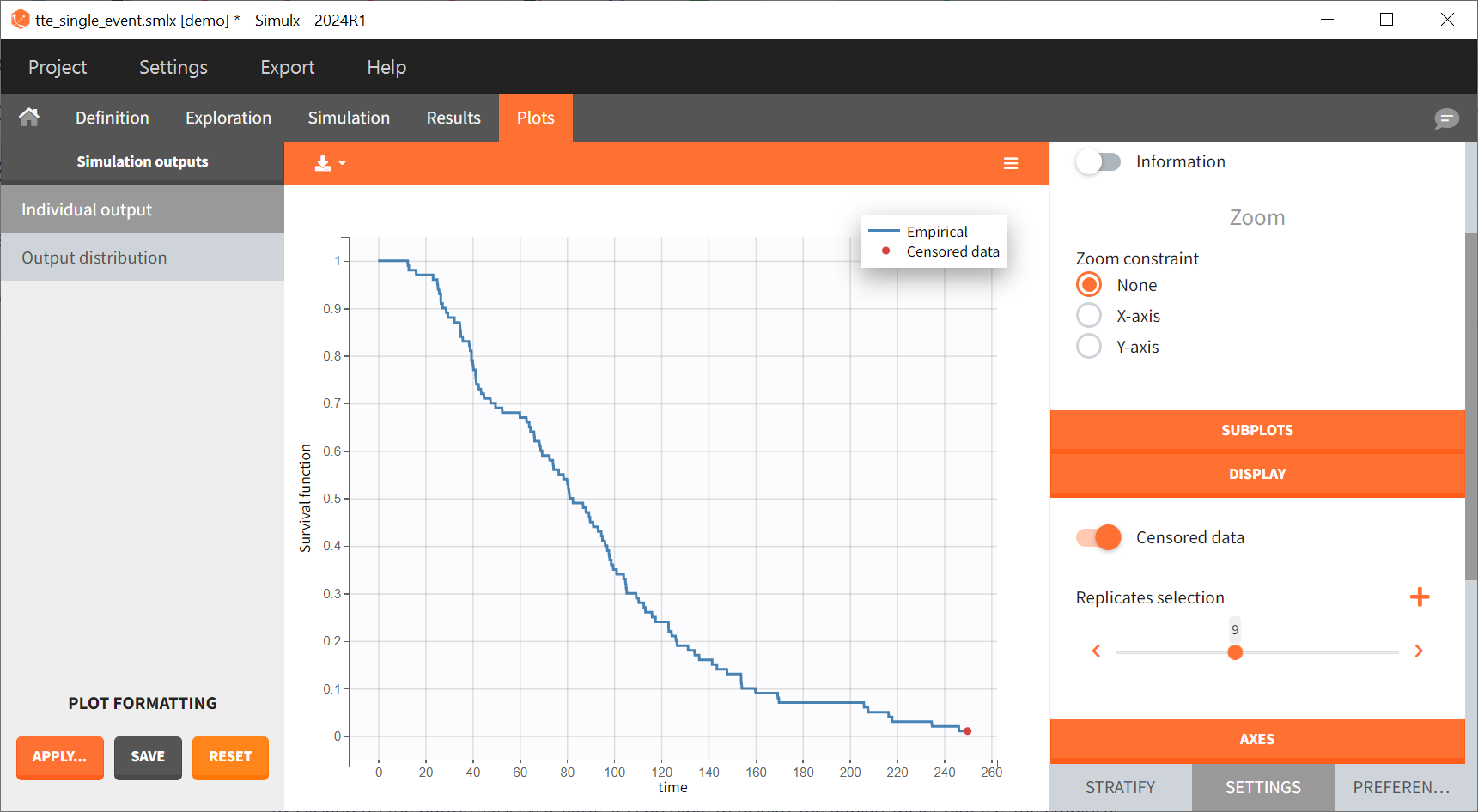
The model is simulated with replicates over 500 subjects until time=250, without inter-individual variability.

Time limits (start time and final time) of the output element define the observation period during which the survival curve is computed. The final time 250 thus defines the censoring time. In the plot Individual output plot, this censoring times is shown as a red dot for some replicates (for example replicate 9 on the figure below) for which some individuals had no event until that time.

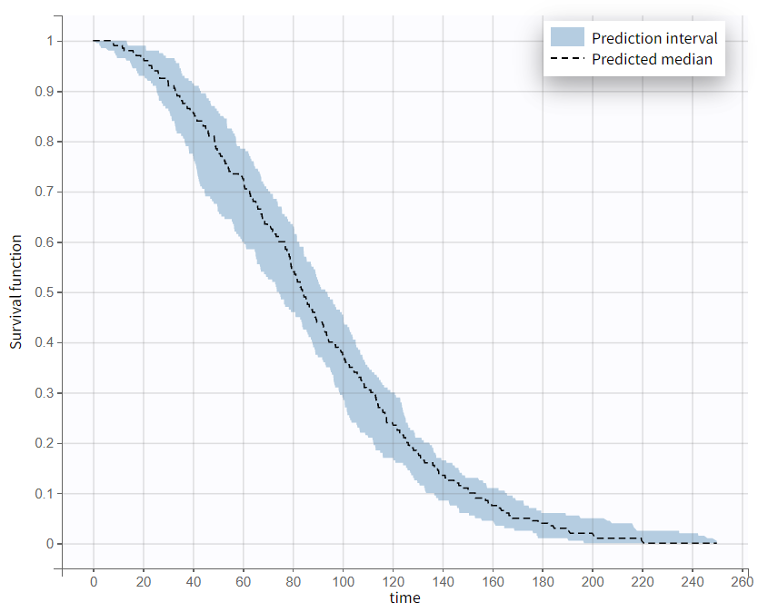
The variability across replicates is visible as a prediction interval on the Output distribution plot:

Single event interval censored or right censored

• 7.1.tte/tte_interval_censored.smlx (model=weibull_model_singleEvent_intCensored_length10.txt)

We may know the event has happened in an interval but not know the exact time . This is interval censoring. 

We use the same basic model, but we now need to specify that the events are interval censored with an interval of length 10:

[LONGITUDINAL]
input = {Te, p}

EQUATION:
h = p/Te * (t/Te)^(p-1)

DEFINITION:
Event = {type=event, maxEventNumber=1, hazard=h, eventType=intervalCensored, intervalLength=10}

OUTPUT:
output = {Event}

Repeated events

Sometimes, an event can potentially happen again and again, e.g., epileptic seizures, heart attacks. For any given hazard function h, the survival function S for individual i now represents the survival since the previous event at , given here in terms of the cumulative hazard from to :

Repeated events exactly observed or right censored

• 7.1.tte/tte_repeated_event.smlx (model=lib:loglogistic_model_repeatedEvents_IIV.txt)

In this demo, a loglogistic TTE model for repeated events, taken from the TTE library and then modified to add IIV on the Te parameter, is simulated over 200 subjects with 50 replicates.

[INDIVIDUAL]
input = {Te_pop, omega_Te}

DEFINITION:
Te = {distribution=logNormal, typical=Te_pop, sd=omega_Te}

[LONGITUDINAL]
input = {Te, s}

EQUATION:
h = s/Te * (t/Te)^(s-1) / (1+(t/Te)^s)

DEFINITION:
Event = {type=event, hazard=h}

OUTPUT:
output = {Event}

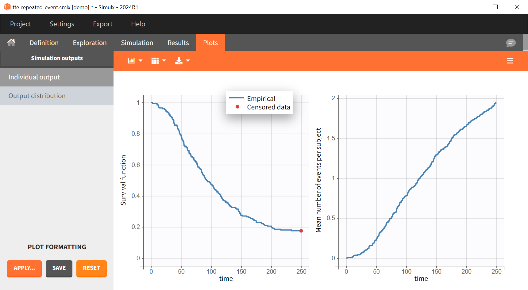
For each simulated individual, a sequence of event times is precisely observed before . The Individual output plots for the first event and the mean number of events per individual is shown for each replicate:

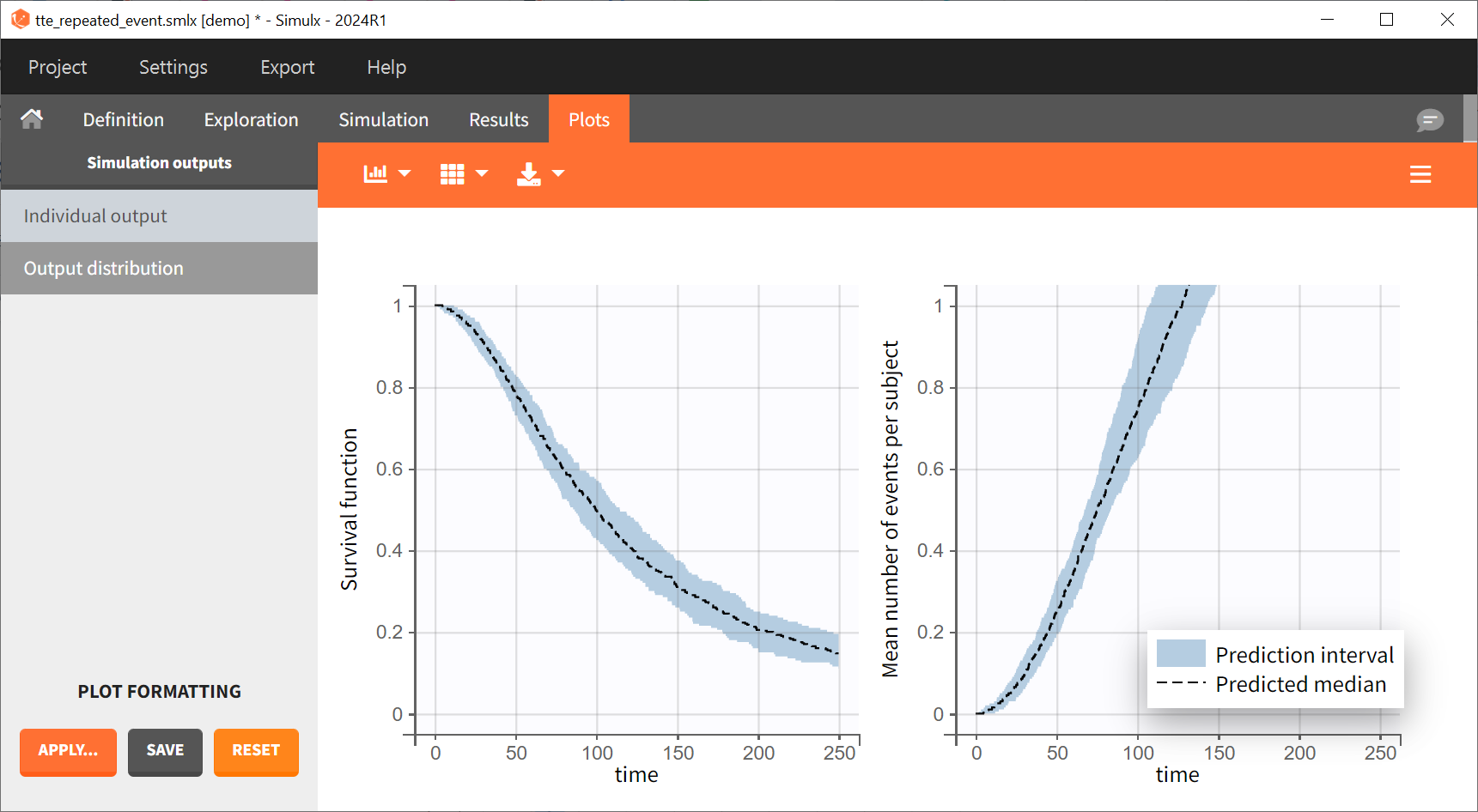
Prediction intervals over all replicates for these two curves are displayed on the Output distribution plot:

Considering the data as count or TTE data

Interval-censored repeated time-to-event data can also be considered as count data: we count the number of events during an interval.

As in Time-to-event observation model , we note the hazard and the cumulative hazard .

Time-to-event data models

The probability density function (pdf) for a single exactly observed event at time is . The pdf for a single event interval-censored between and , is . The pdf for repeated interval censored events is slightly more complicated.

The probability density function (pdf) to observe events within a time interval from to , given the hazard , can be calculated as:

with being the cumulative hazard between and .

If we have a model with a constant hazard , the cumulative hazard is equal to and the probability density function is:

If, in addition, the intervals over which the events are counted are all of equal length, then we can define and obtain:

We recognize the usual Poisson model for count data, which assume independent events and equal interval durations.

If we want to write a count model for data with non-equal interval durations, we can still use the Poisson model but make sure that the parameter takes into account the interval duration. This can be done by passing the interval duration as REGRESSOR, or by passing as REGRESSOR and obtaining the time , which is the current time, using the mlxtran keyword t.

The models for the data considered as TTE and the model for the data considered as count are equivalent. Note that when defining a TTE model, it is the hazard that must be defined. When defining the count model, we define the pdf. Thus, considering the data as count can also be used to model TTE data but provide a custom likelihood (pdf) instead of providing the hazard function.

Model parameters should be consistent whether the data is considered as count or as TTE. However the plots provided by Smulx will be different: survival curve in case of TTE and probability over time to observed k events in case of count data.

A detailed example of a dataset modeled either with a TTE model or a count model is shown on the Monolix documentation page, these projects can be easily exported to Simulx and simulated to see the difference there.

Formatting of time-to-event data in the MonolixSuite

Exporting simulated events in Simulx will generate a time-to-event dataset. This section explains how such data is formatted in the MonolixSuite.

In the data set, exactly observed events, interval censored events and right censoring are recorded for each individual. Contrary to other softwares for survival analysis, the MonolixSuite requires to specify the time at which the observation period starts. This allows to define the data set using absolute times, in addition to durations (if the start time is zero, the records represent durations between the start time and the event).

The column TIME also contains the end of the observation period or the time intervals for interval-censoring. The column OBSERVATION contains an integer that indicates how to interpret the associated time. The different values for each type of event and observation are summarized in the table below:

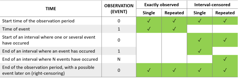
The figure below summarizes the different situations with examples:

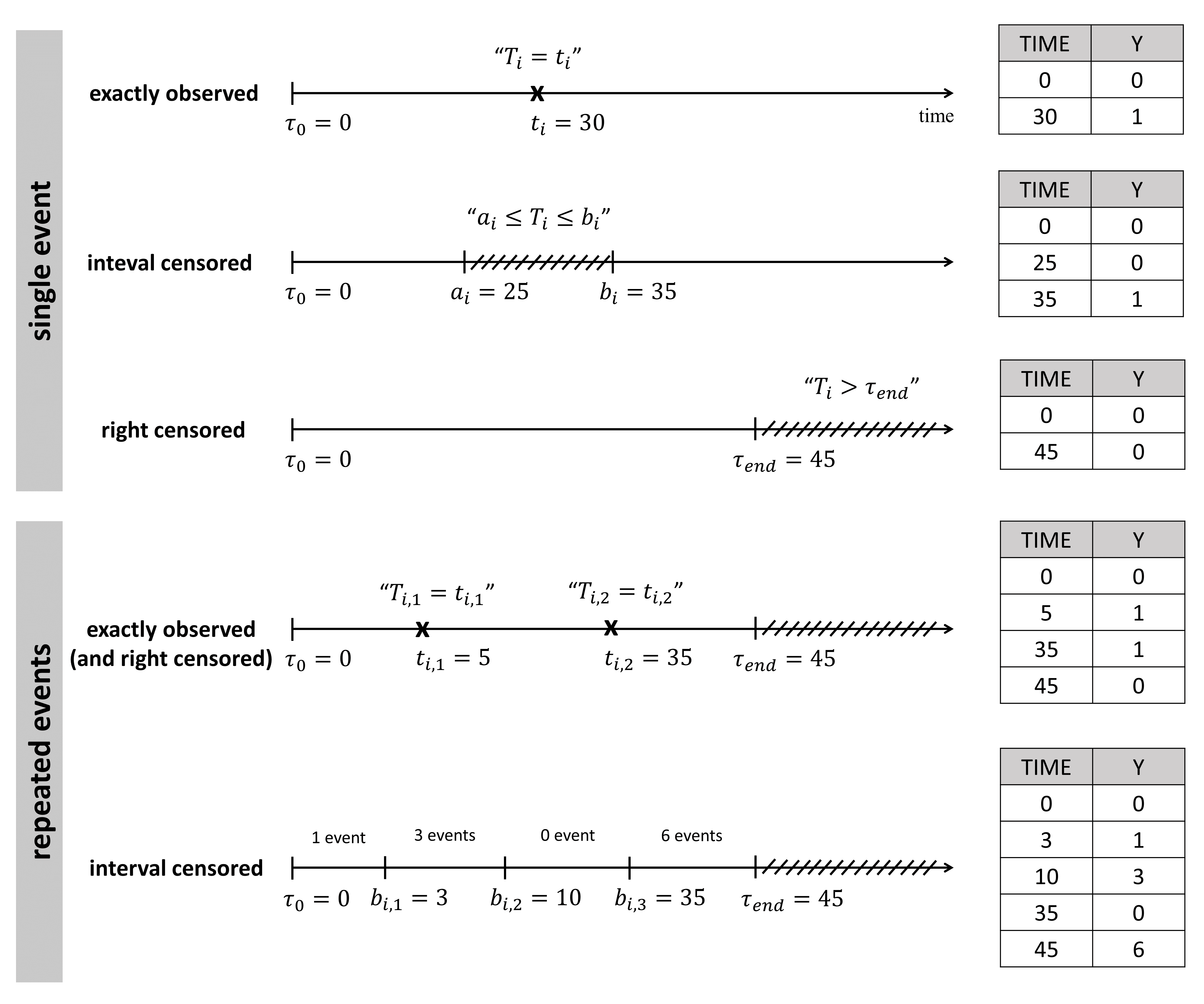
For instance for single events, exactly observed (with or without right censoring), one must indicate the start time of the observation period (Y=0), and the time of event (Y=1) or the time of the end of the observation period if no event has occurred (Y=0). In the following example:

ID TIME Y
1   0   0
1  34   1
2   0   0
2  80   0

the observation period lasts from starting time t=0 to the final time t=80. For individual 1, the event is observed at t=34, and for individual 2, no event is observed during the period. Thus it is noticed that at the final time (t=80), no event had occurred. Using absolute times instead of duration, we could equivalently write:

ID TIME Y
1  20   0
1  54   1
2  33   0
2  113  0

The duration between start time and event (or end of the observation period) are the same as before, but this time we record the day at which the patients enter the study and the days at which they have events or leave the study. Different patients may enter the study at different times.

Examples for repeated events, and interval censored events are available on the Monolix data set documentation page.