Initialization of parameters

Parameters of the model you defined in the MODEL tab are listed in the RUN tab under Settings. Each parameter has two attributes: an initial value and a constraint.

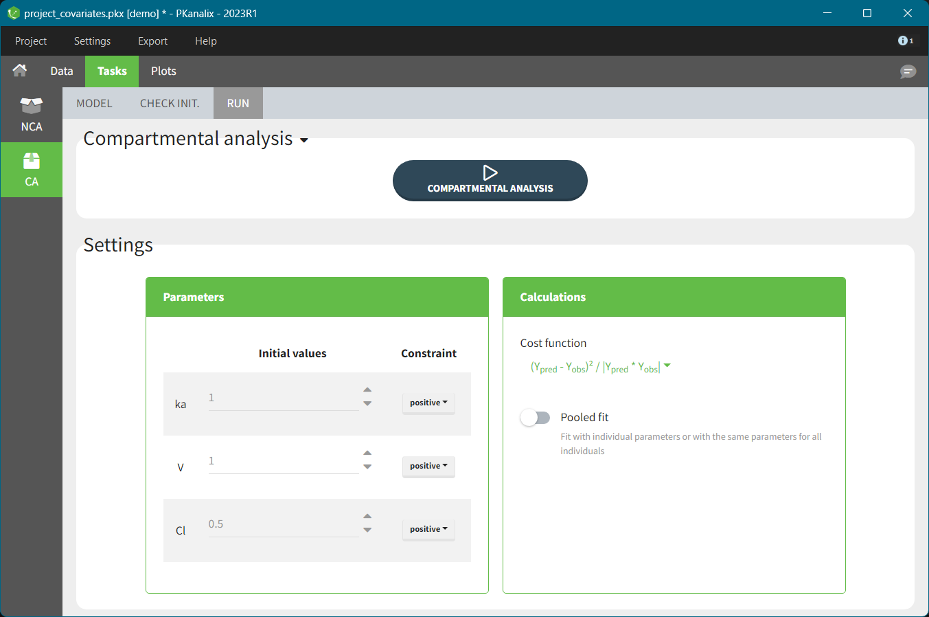
Constraints set a range of allowed values for selected parameter during estimation (and as initial values). There are three types of constraints:

• none: a parameter is not constraint and its value can be from minus to plus “infinity” (in practice its minus or plus 10e16),

• positive: (default option) a parameter is strictly greater then zero,

• bounded: a parameter is strictly inside a bounded interval which limits you can specify manually.

You can set an initial value of a parameter manually or using the auto-initialization algorithm. Selection of good initial values, those capturing the characteristic features of a selected model (e.g., two different slopes on log scale for a 2-compartment model), is important during the estimation of parameters with the optimization algorithm. It can help to avoid local minima during the optimization process and decrease the runtime of the algorithm.

Check initial estimates

In the Tasks tab of the CA section, there is a dedicated sub-tab CHECK INIT. to help with the initialization of parameters. The goal of the CHECK INIT. sub-tab is to:

• Visually check parameter initialization. It displays the model predictions obtained with the initial model parameters values and the individual designs (doses and regressors) for each individual and the data points for comparison.

• Help finding good initial values: update the values manually or use the auto-init function.

The CHECK INIT. tab in PKanalix uses the same auto-init algorithm and has the same features as auto-init in Monolix.

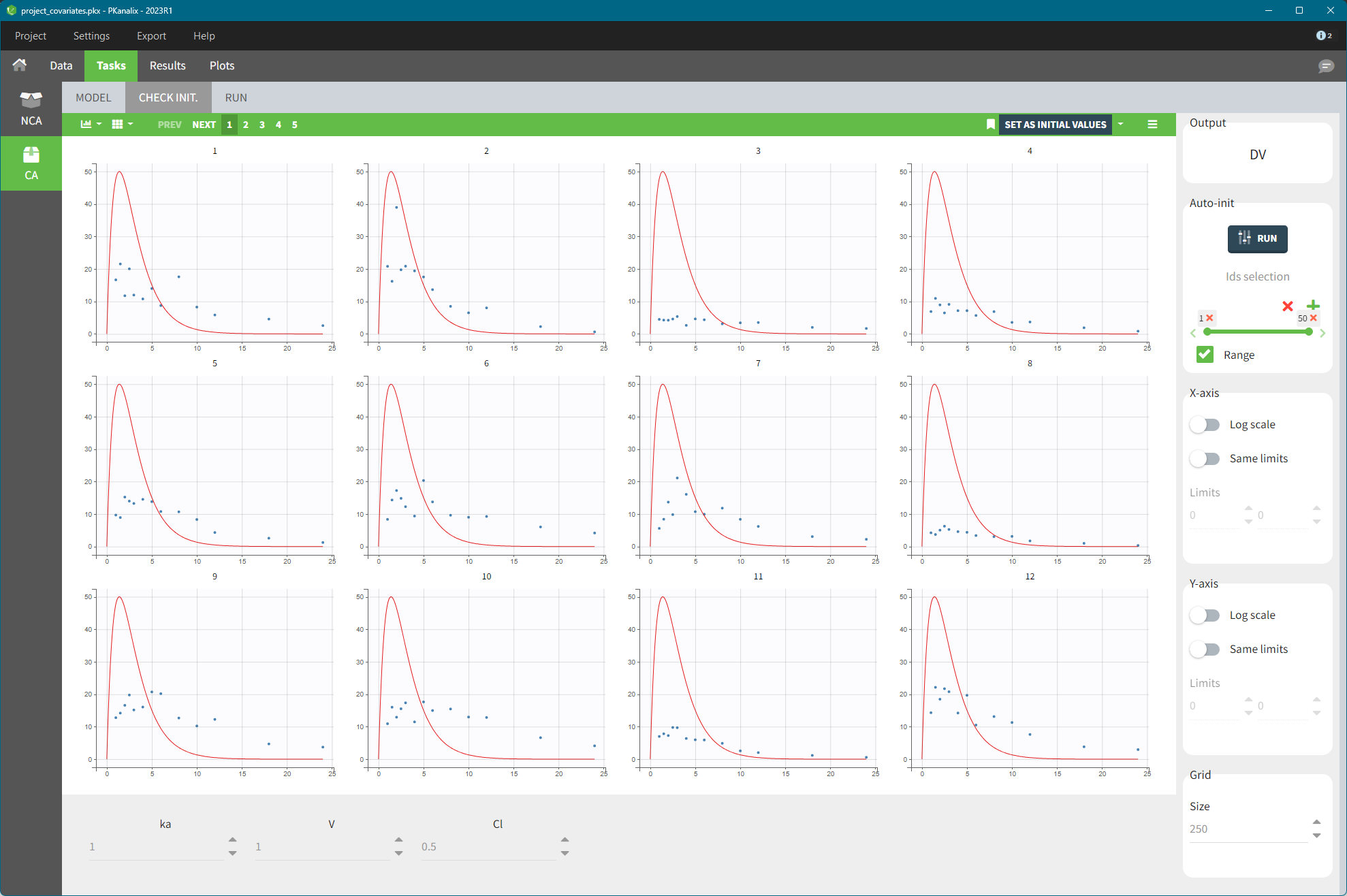
The panel on the right side contains several settings:

• Auto-init: You can modify the initial values of the parameters, shown on the bottom of the screen, manually by typing new values or by using the auto-init algorithm–click the button RUN in the Auto-init panel on the right. See more details below.

• X-axis and Y-axis: Set one or both axes to log-scale. To better compare among individuals, apply the same limits for all individual plots.

• Grid: If there are not enough points for the prediction (e.g. there are many doses), change the grid size by increasing the number of points.

Click on the “SET AS INITIAL VALUES” button on the top of the plot to save the initial values for the optimization step.

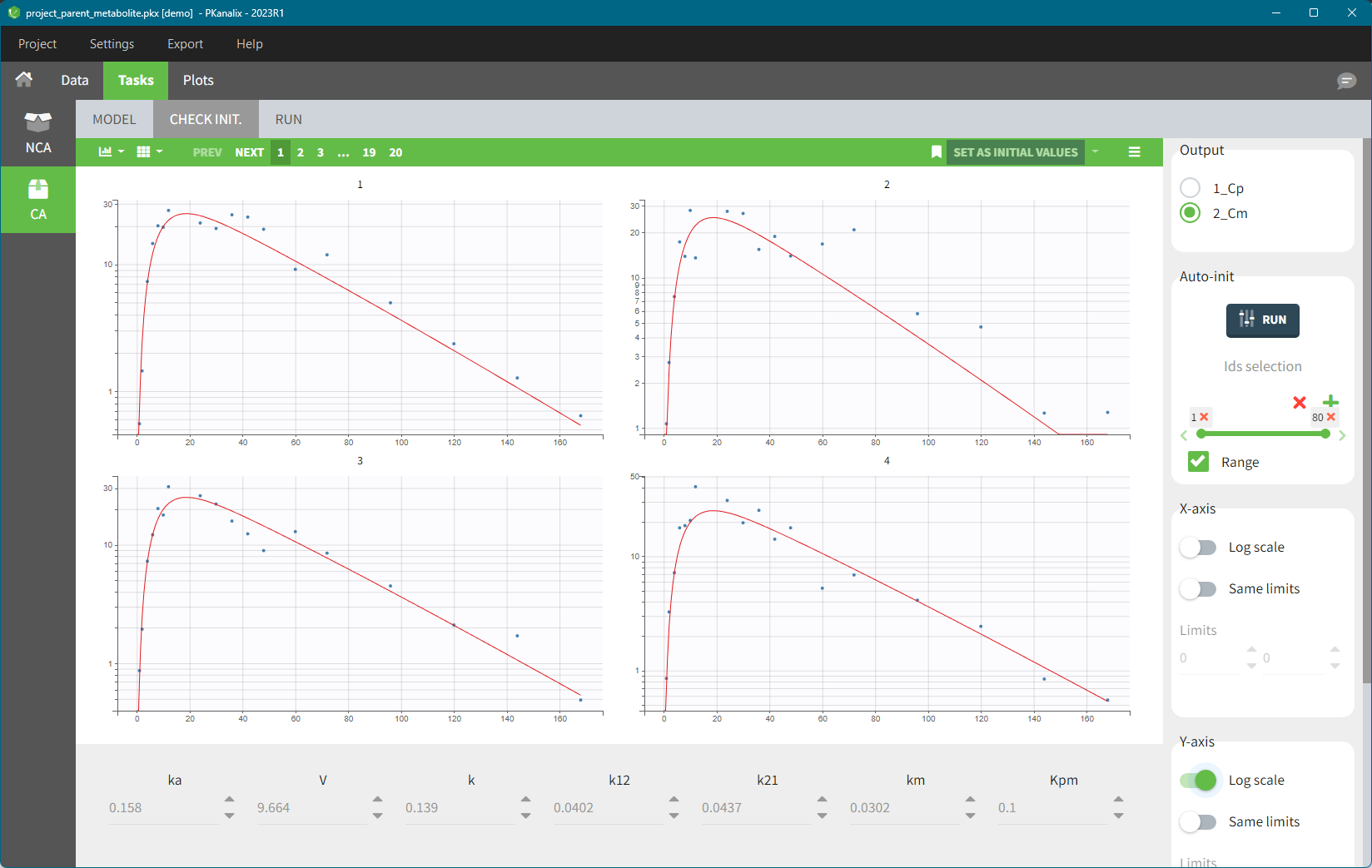
If there are several observation types where the different obs-ids have been mapped to model outputs (for example, a parent and a metabolite, or a PK and a PD observation), then you can switch between them in the “Output” section on the top-right corner, see below:

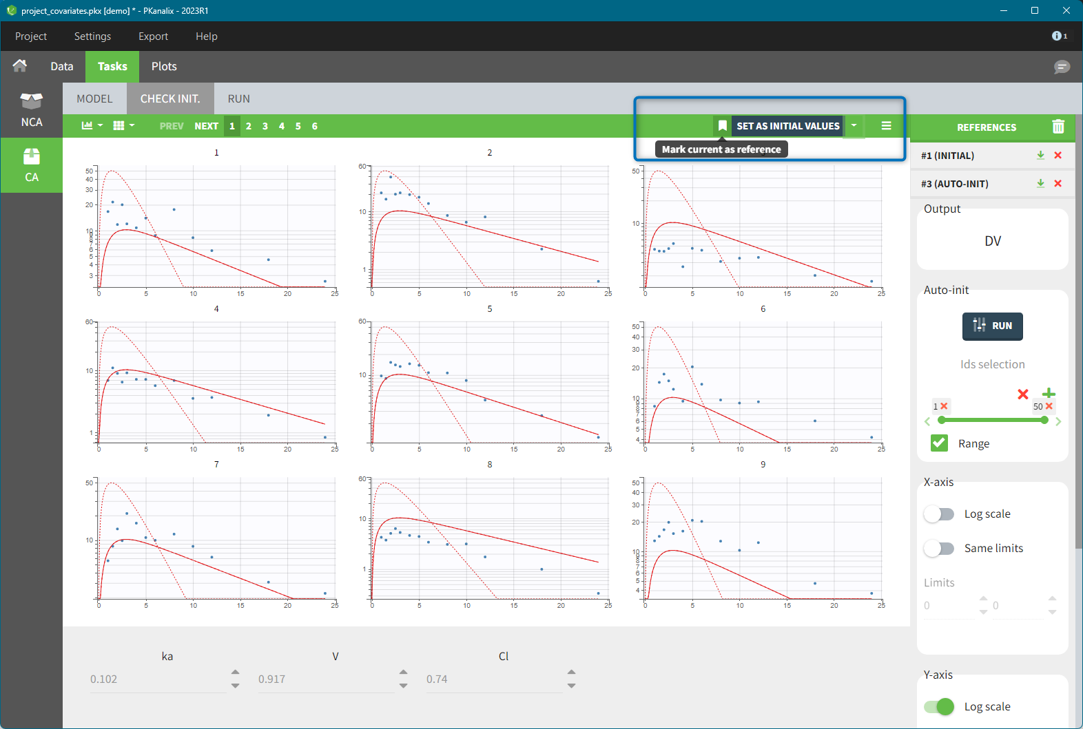
References in the “check initial estimates”

The following video describes how to use the Reference option and when it can be helpful (the example is in Monolix, but it works in the same way in PKanalix).

Adding a reference better shows how changing parameter values impacts the prediction. To add a reference, click on the icon to the left “Set as initial values” button. It saves the current parameter values as a reference and adds it to the list at the top of the right panel, see below. If you then further change the parameter values either manually or with auto-int, the solid red curve corresponds to the new current set of parameters (displayed at the bottom), while the dashed one corresponds to the reference. At any time, you can restore the reference as the current parameter values (green arrow next to the reference name), delete the reference (red x) or delete all references (trash icon above the list).

Auto-init: Automatic initialization of the parameters

PKanalix has an automatic algorithm for initialization. It is in the right panel in the Auto-init section and you can launch it by clicking on the button RUN. The following video describes how it works using an example in Monolix.

After clicking on the button RUN, PKanalix computes initial model parameters that best fit the data points using a pooled-fit approach, starting from the current parameter values displayed at the below the plots. By default, the algorithm uses all individual data from all observations mapped to a model output. You can change the set of individuals in the “Ids” selection panel just below the RUN button.

The algorithm is a custom optimization method on the pooled data. The purpose is not to find a perfect match but rather to have all the parameters in a good range for starting the Nelder-Mead optimization on each individual.

• While auto-init is running, the pop-up shows the evolution of the cost of the optimization algorithm over the iterations. Stop the algorithm at any time, e.g., if you see that the cost has decreased sufficiently and you want to check the parameter values.

• Note that the more individuals you select, the longer the run will take.

• Selecting one or only a few individuals that show clearly model characteristics (e.g., a third compartment, a complex absorption) can help the auto-init algorithm to find set of parameters that is sensitive to specific model features.

After running auto-init, the current parameter values update automatically and are shown in the plots. To use these parameters as initial values forthe optimization process, click on the button “SET AS INITIAL VALUES.”

Note that the auto-init procedure uses the current initial values. If it gives poor results, manually change the parameter values before running the auto-init again.