Examples

Bioavailability

Bioavailability

This example shows how to calculate absolute bioavailability from NCA parameters in PKanalix.

https://youtu.be/3klneQooms0?feature=shared

Introduction

The bioavailability is the percentage (fraction) of the administered drug amount that reaches the systemic circulation.

• Intravenous administration: bioavailability = 100% as you inject the totality of the drug directly in the systemic circulation.

• Extravascular administration (oral or subcutaneous): bioavailability < 100% as part of a dose will be lost before reaching the bloodstream. For instance, for an oral dose, the drug needs to cross the intestinal wall or be processed by the liver before reaching the systemic circulation. Only a fraction of the dose will remain after these steps. 

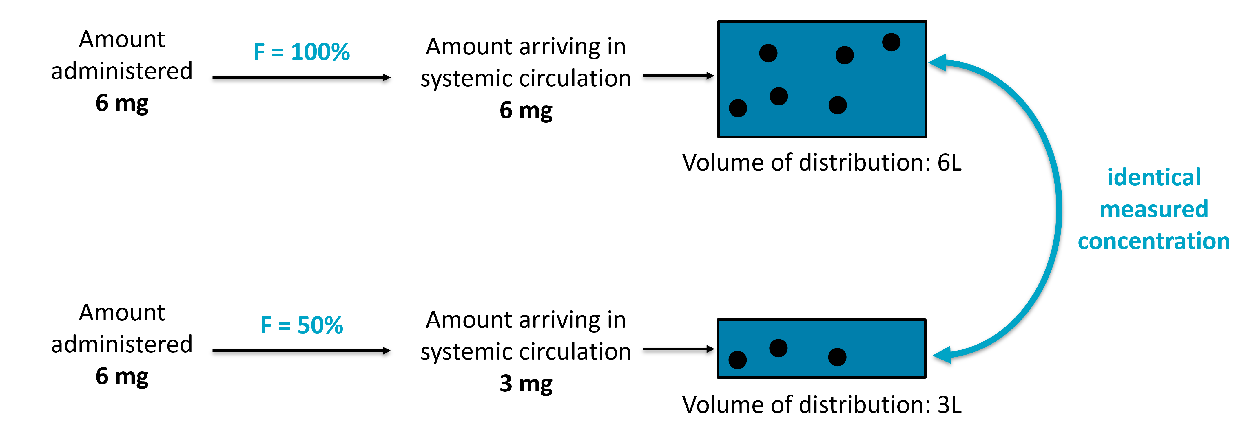
If you have only extravascular data, it is not possible to calculate the absolute bioavailability because it’s not possible to identify both the absorption percentage and the volume in which it is absorbed. In other words, the concentration observed in the blood would be the same  for a large fraction of the dose absorbed and a small volume of distribution, or on the  other hand, for a small fraction absorbed and a large volume of distribution - see figure below. 

However, with a PK data with both extravascular and intravenous doses, it is possible to calculate the absolute bioavailability by comparing the total exposure in both cases. The following example uses an oral dose, but the same methodology applies for other extravascular routes.

Definition of bioavailability

The typical formula to calculate the bioavailability is:

with representing the total exposure. The AUC to infinity is proportional to the amount of drug that reaches the circulation, up to a constant beta we don’t know. By using the ratio, the unknown constant cancels out. And for IV, the amount that reaches the circulation is equal to the amount of the administered dose. If the dose amount is the same for IV and Oral, I get the fraction of the dose amount that reaches the circulation compared to the amount administered.

This formula works if I use the same administered dose for the oral and iv route. If not, we can adapt the formula by normalizing by the dose amount for both routes. The denominator cancels out and I obtain the same as above. 

The general formula to calculate the bioavailability in a common notation for the dose amount is: 

We will distinguish two cases:

Case 1: Parallel design

Each individual has received only one of the two formulations in a parallel design. We can calculate only an average bioavailability by doing the ratio of the average for oral over average for iv. This can be done using the bioequivalence module. The result is the ratio and the confidence interval.

Case 2: Crossover design

Each individual has received both oral and IV formulations in several periods. We can calculate the bioavailability for each individual using the ratio module. We can also calculate an average bioavailability and its confidence interval using the BE module like the first case.

Parallel design

Demo project: 3.bioequivalence/project_parallel_absBioavailability

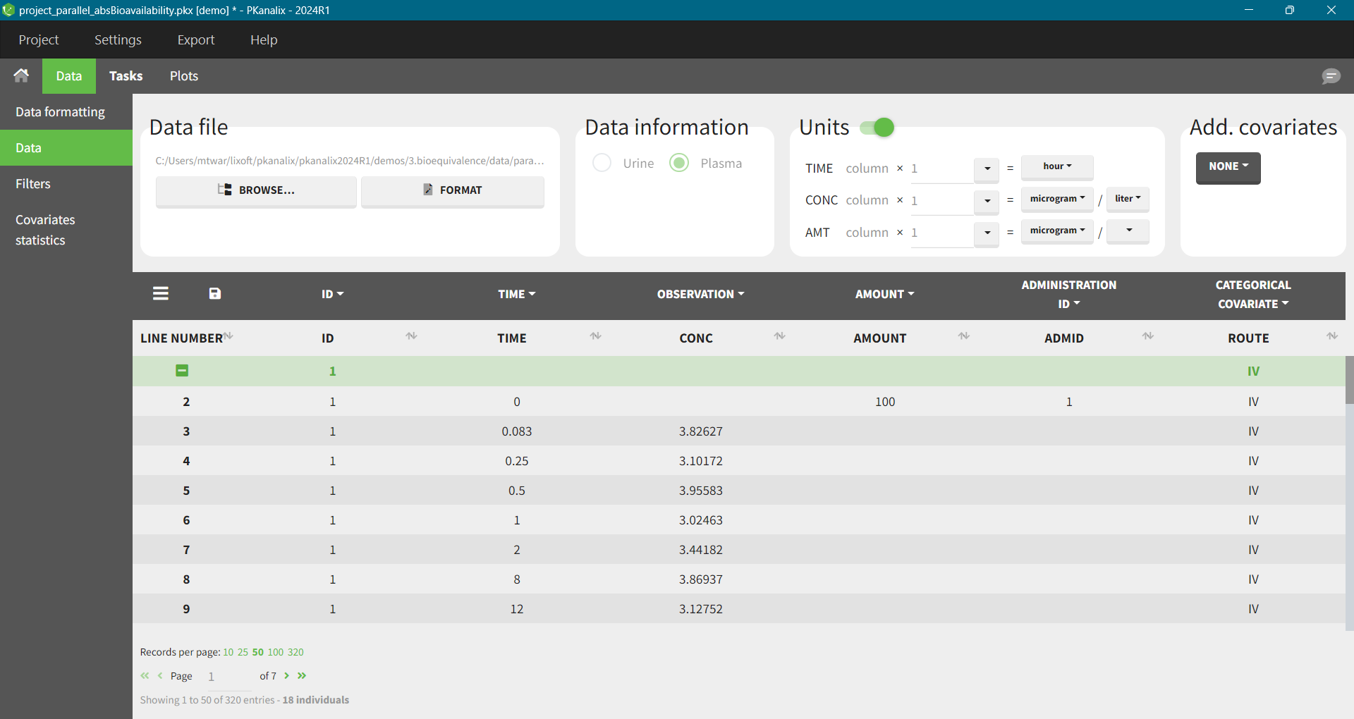
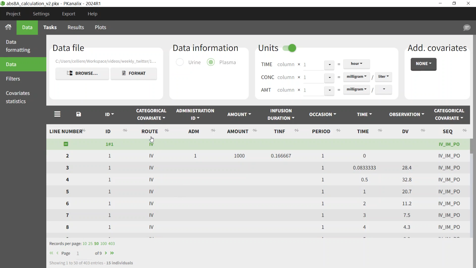
In this project half of the individuals have received an oral dose and half an intravenous dose. It is necessary to have in the dataset a column to distinguish the two routes - mapped as categorical covariate. Column ADMID mapped as “Administation ID” will distinguish the two types of doses.

To account for different doses in the formula, we can use the dose normalized AUC to infinity (AUCinf_D) to calculate F.

In the settings:

• administration type: 1 = intravenous, 2 = extravascular. This will impact the formula used for some of the NCA parameters.

• parameters: AUCINF_D. This parameter will be used in the bioequivalence module to calculate the bioequivalence, so the box in the BE column must be selected. By default “log-transform” is applied, which means that I will calculate the average for each route as a geometric mean.

BE module:

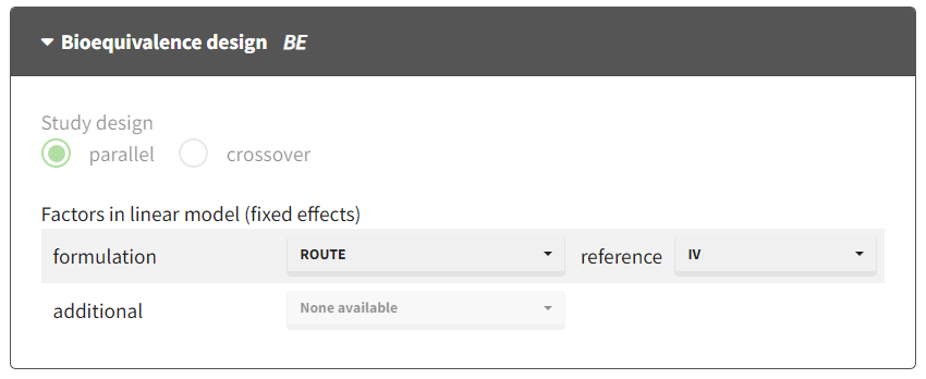
• the design is automatically recognized as parallel

• the ratio will be calculated using the categorical covariate indicated on the line “formulation”: select the ROUTE column from the dataset

• the reference is set to IV (denominator)

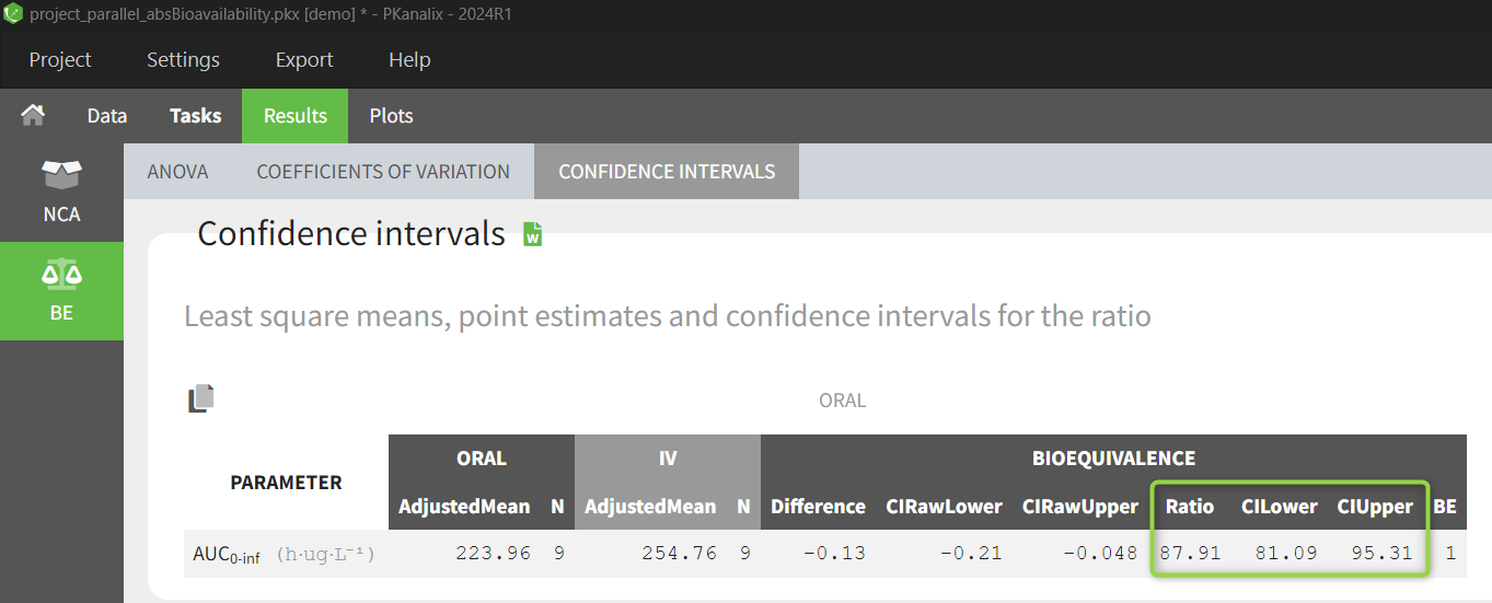
Results show the calculated bioavailability in the confidence interval table - the ratio is in percentage.

Crossover design

In a crossover design with several periods we can have one or several sequences. It does not change the calculation. What is important is to have several periods for each individual, one with the IV formulation and one with the extravascular formulation.

In the example each individual has 3 periods, one IV, one intramuscular and one oral. The PERIOD column must be mapped as occasion - PKnalix will detect each period as a separate profile to analyze.

The NCA settings are set similarly to the previous example, the dose-normalized AUC is selected as the parameter.

BE module:

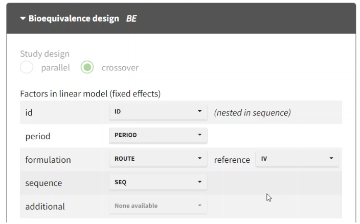
• crossover design is detected automatically

• include ROUTE as the formulation with IV as a reference

• include the PERIOD and SEQUENCE columns as factors in the linear model to account for any effect they may have on the exposure. 

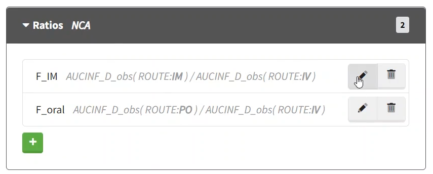
Individual bioavailability

In addition to the average bioavailability, we can calculate the bioavailability for each individual, as a ratio of the individual AUCINF_D of:

• IM versus IV

• Oral versus IV

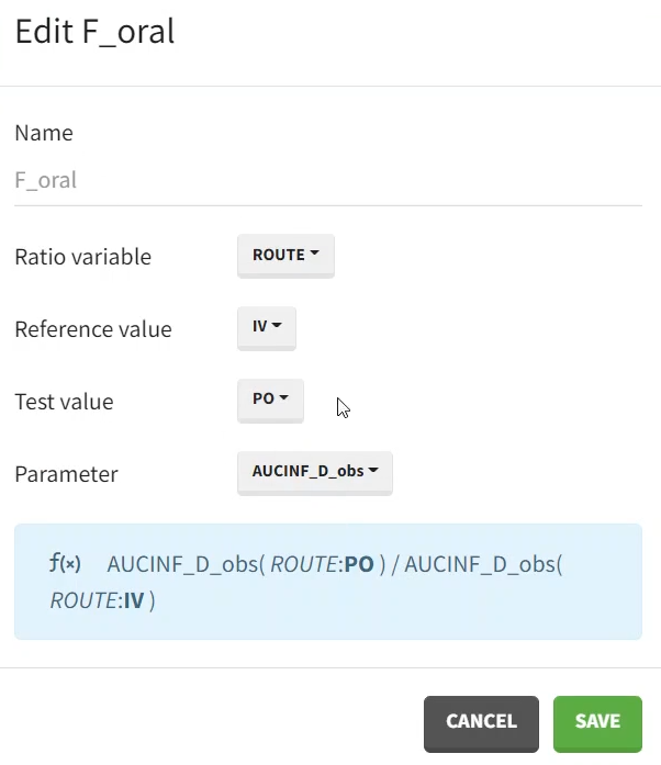
It can be calculated using the ratio feature - available in case of occasions. In the pop-up window, we define:

• a name, for instance F_oral,

• the variable for which the ratio is defined, here ROUTE

• the reference (in the denominator): IV and the test (nominator): PO.

• parameter: AUCINF_D_obs

The same can be done for the IM formulation.

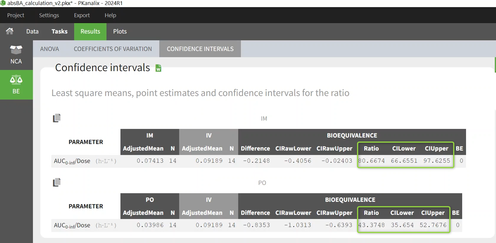
In the results, in the BE section, the average bioavailability is shown as a percentage calculated using the linear model, with the confidence interval.

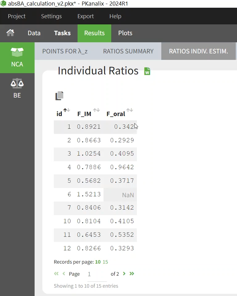
In the Results/NCA/Ratio there is the bioavailability for each formulation and each individual as a ratio between 0 and 1.

The Ratio summary table includes the descriptive statistics of the ratio over all individuals. Note that in the current 2024 version of PKanalix, it is not possible to stratify the ratio summary table.

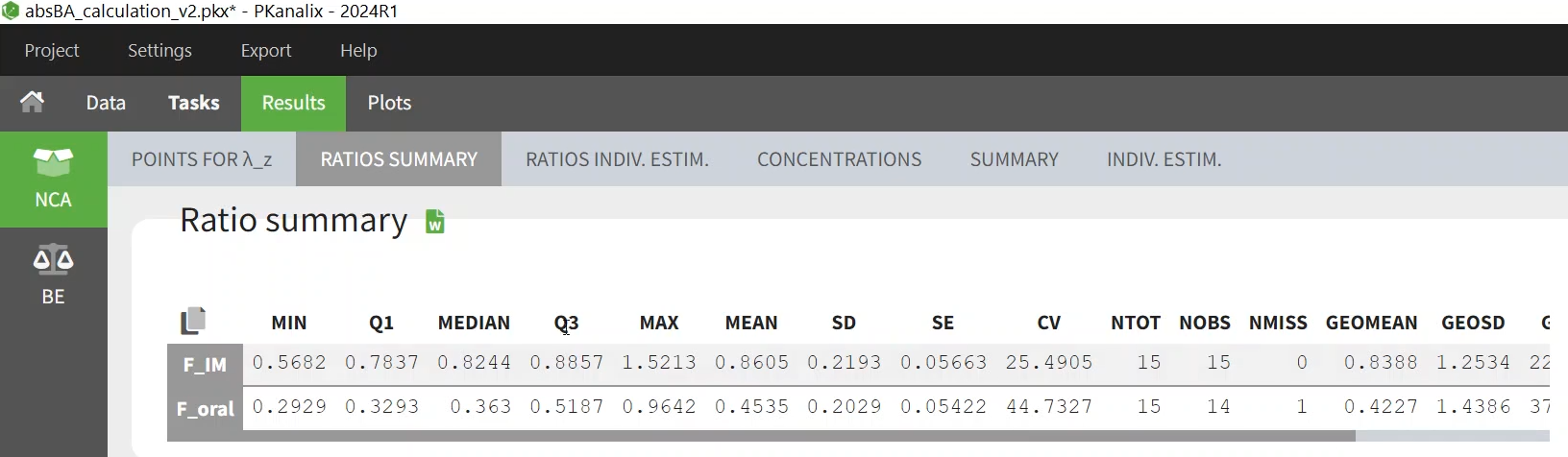
The geometric mean here can differ from the value in the BE tab, because one is the geometric mean of the individual ratios, while the other is the ratio of the geometric means. In addition, here the values are corrected for a possible period and sequence effect.