Using regressors

Objectives: learn how to define and use regression variables (time varying covariates).

Demos: reg1_project, reg2_project

Introduction

A regression variable is a variable x which is a given function of time, which is not defined in the model but which is used in the model. x is only defined at some time points (possibly different from the observation time points), but x is a function of time that should be defined for any t (if is used in an ODE for instance, or if a prediction is computed on a fine grid). Then, Mlxtran defines the function x by interpolating the given values . In the current version of Mlxtran, interpolation is performed by using the last given value:

Or linearly:

Regressor definition in a data set

It is possible to have in a data set one or several columns with column-type REGRESSOR. Within a given subject-occasion, string “.” will be interpolated (last value carried forward interpolation is used) for observation and dose-lines. Lines with no observation and no dose but with regressor values are also taken into account by Monolix for regressor interpolation.

Several points have to be noticed:

• The name of the regressor in the data set and the name of the regressor used in the longitudinal model do not need to be identical.

• If there are several regressors, the mapping will be done by order of definition.

• Regressors can only be used in the longitudinal model.

Continuous regression variables

• reg1_project (data = reg1_data.txt , model=reg1_model.txt)

We consider a basic PD model in this example, where some concentration values are used as a regression
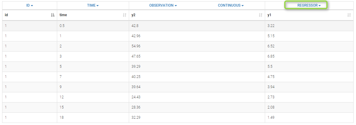
variable. The data set is defined as follows

[LONGITUDINAL]
input = {Emax, EC50, Cc}
Cc    = {use=regressor}

EQUATION:
E = Emax*Cc/(EC50 + Cc)

OUTPUT:
output = E

As explained in the previous subsection, there is no name correspondance between the regressor in the data set and the regressor in the model file. Thus, in that case, the values of Cc with respect to time will be taken from the y1 column.
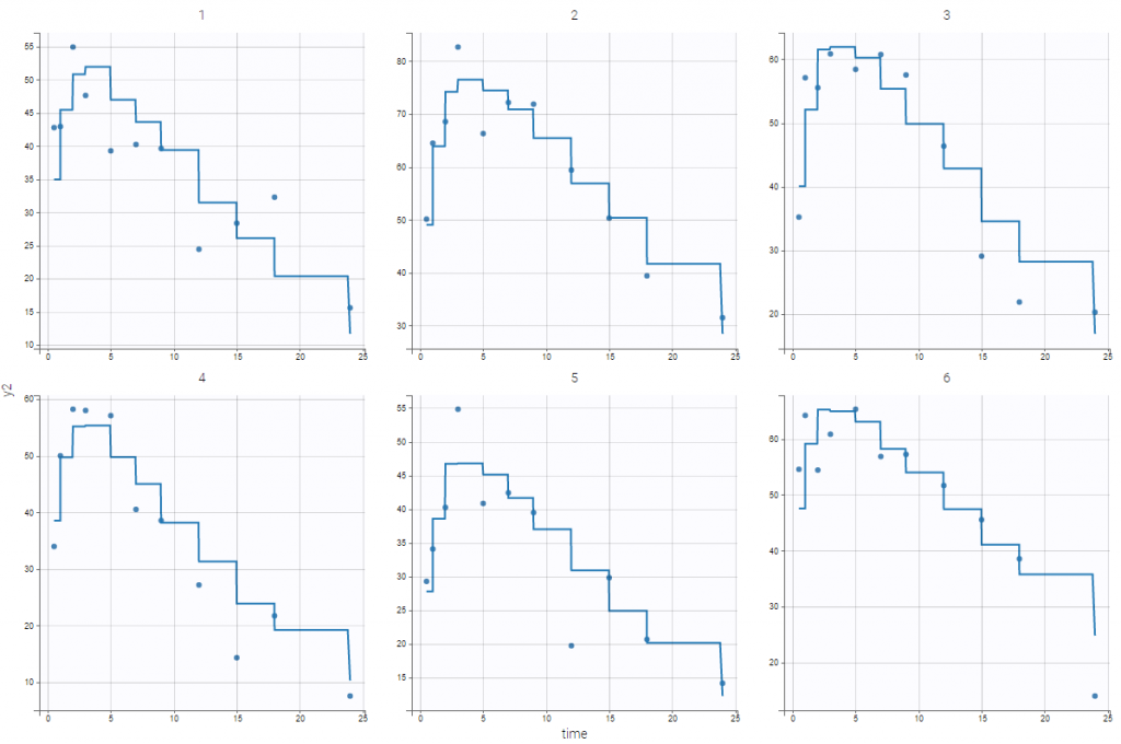
In addition, in that case, the predicted effect is therefore piece wise constant because

• the regressor interpolation is performed by using the last given value, and then Cc is piece wise constant.

• The effect model is direct with respect to the concentration.

Thus, it changes at the time points where concentration values are provided:

Categorical regression variables

• reg2_project (data = reg2_data.txt , model=reg2_model.txt)

The variable takes its values in {1, 2} in this example and represents the state of individual i at time . We then assume that the observed data has a Poisson distribution with parameter lambda1 if and parameter lambda2 if . z is known in this example: it is then defined as a regression variable in the model:

[LONGITUDINAL]
input = {lambda1, lambda2, z}
z = {use=regressor}
                           
EQUATION:
if z==0
   lambda=lambda1
else
   lambda=lambda2
end

DEFINITION:
y = {type=count, 
     log(P(y=k)) = -lambda + k*log(lambda) - factln(k)
}

OUTPUT:
output = y