Time-to-event data models

Related resources on modeling time-to-event data in Monolix:

• Columns used to define observations: formatting of time-to-event data in the MonolixSuite.

• Time-to-event observation model : details on the different models for time-to-event data that can be used in Monolix and their syntax.

• Time-to-event model library : detailed description of the library of time-to-event models integrated within Monolix.

On the current page, we show examples of time-to-event data models from the Monolix demos, and we then discuss how interval-censored repeated time-to-event data can also be considered as count data with examples in Monolix.

Demos: tte1_project, tte2_project, tte3_project, tte4_project, rtteWeibull_project, rtteWeibullCount_project

Single event

To begin with, we will consider a one-off event. Depending on the application, the length of time to this event may be called the survival time (until death, for instance), failure time (until hardware fails), and so on. In general, we simply say “time-to-event”. The random variable representing the time-to-event for subject i is typically written Ti.

Single event exactly observed or right censored

• tte1_project (data = tte1_data.txt , model=lib:exponential_model_singleEvent.txt)

The event time may be exactly observed at time , but if we assume that the trial ends at time , the event may happen after the end. This is “right censoring”. Here, Y=0 at time t means that the event happened after t and Y=1 means that the event happened at time t. The rows with t=0 are included to show the trial start time :
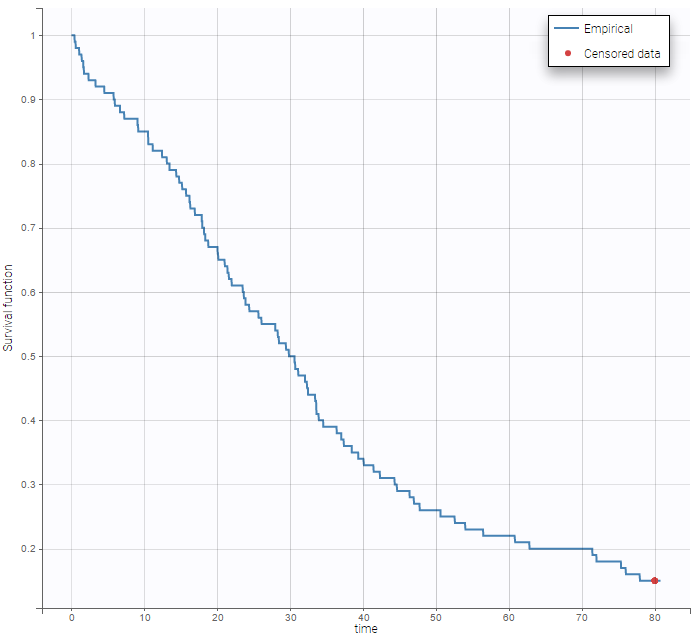
By clicking on the button Observed data, it is possible to display the Kaplan-Meier plot (i.e. the empirical survival function) before fitting any model:

A very basic model with constant hazard is used for this data:

[LONGITUDINAL]
input = Te
  
EQUATION:
h = 1/Te

DEFINITION:
Event = {type=event, maxEventNumber=1, hazard=h}

OUTPUT:
output = {Event}

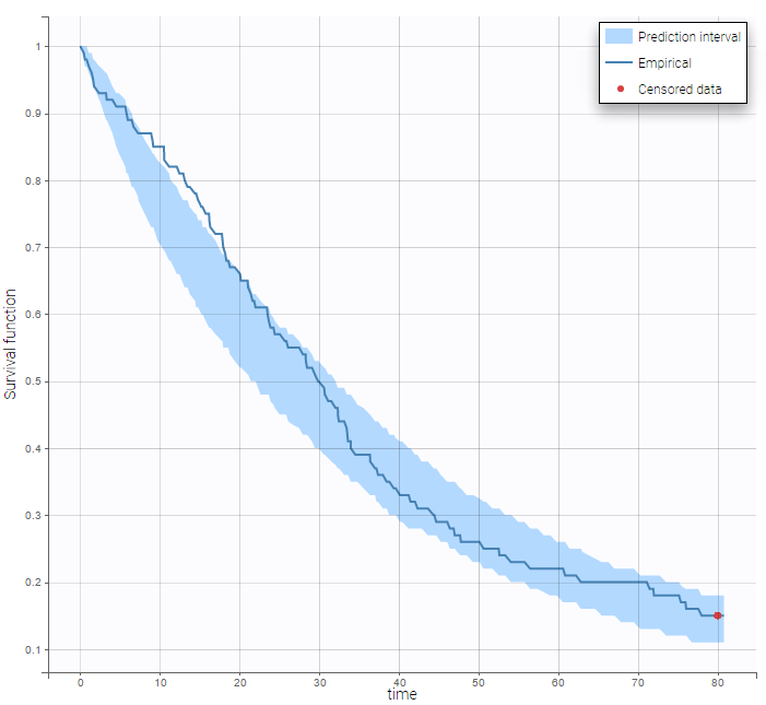
Here, Te is the expected time to event. Specification of the maximum number of events is required both for the estimation procedure and for the diagnosis plots based on simulation, such as the predicted interval for the Kaplan Meier plot which is obtained by Monte Carlo simulation:

Single event interval censored or right censored

• tte2_project (data = tte2_data.txt , model=exponentialIntervalCensored_model.txt)

We may know the event has happened in an interval but not know the exact time . This is interval censoring. Here, Y=0 at time t means that the event happened after t and Y=1 means that the event happened before time t.
Event for individual 1 happened between t=10 and t=15. No event was observed until the end of the experiment (t=100) for individual 5. We use the same basic model, but we now need to specify that the events are interval censored:

[LONGITUDINAL]
input = Te  

EQUATION:
h = 1/Te

DEFINITION:
Event = {type=event, maxEventNumber=1, eventType=intervalCensored, hazard = h
         intervalLength=5     ; used for the plots (not mandatory)
}

OUTPUT:
output = Event

Repeated events

Repeated events exactly observed or right censored

• tte3_project (data = tte3_data.txt , model=lib:exponential_model_repeatedEvents.txt)

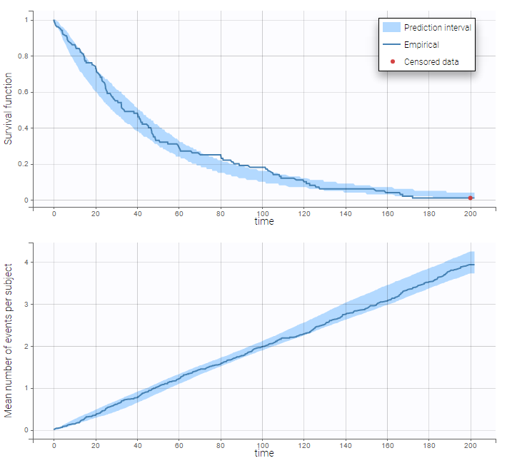
A sequence of event times is precisely observed before : We can then display the Kaplan Meier plot for the first event and the mean number of events per individual:

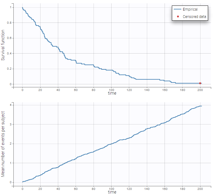
After fitting the model, prediction intervals for these two curves can also be displayed on the same graph as on the following: 

Repeated events interval censored or right censored

• tte4_project (data = tte4_data.txt , model=exponentialIntervalCensored_repeated_model.txt)

We do not know the exact event times, but the number of events that occurred for each individual in each interval of time.

Considering the data as count or TTE data

Interval-censored repeated time-to-event data can also be considered as count data: we count the number of events during an interval.

Link between TTE models and count models

As in Time-to-event observation model , we note the hazard and the cumulative hazard .

The probability density function (pdf) for a single exactly observed event at time is . The pdf for a single event interval-censored between and , is . The pdf for repeated interval censored events is slightly more complicated.

The probability density function (pdf) to observe events within a time interval from to , given the hazard , can be calculated as:

with being the cumulative hazard between and .

If we have a model with a constant hazard , the cumulative hazard is equal to and the probability density function is:

If, in addition, the intervals over which the events are counted are all of equal length, then we can define and obtain:

We recognize the usual Poisson model for count data, which assume independent events and equal interval durations.

If we want to write a count model for data with non-equal interval durations, we can still use the Poisson model but make sure that the parameter takes into account the interval duration. This can be done by passing the interval duration as REGRESSOR, or by passing as REGRESSOR and obtaining the time , which is the current time, using the mlxtran keyword t.

The models for the data considered as TTE and the model for the data considered as count are equivalent. Note that when defining a TTE model, it is the hazard that must be defined. When defining the count model, we define the pdf. Thus, considering the data as count can also be used to model TTE data but provide a custom likelihood (pdf) instead of providing the hazard function.

Estimated model parameters should be consistent whether the data is considered as count or as TTE. However the diagnostic plots provided by Monolix will be different: Kaplan-Meier curve in case of TTE and probability over time to observed k events in case of count data.

Below we show an example with the more complex Weibull model.

Example with a Weibull model

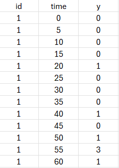
The following dataset will be used with both approaches (TTE and count). As can be seen for individual 1, some intervals have 0 events, some 1 and some several (e.g 3). The number of observed events is indicated as an integer in the Y column tagged as OBSERVATIONS.

• weibullRTTE (data = weibull_data.txt , model=weibullRTTE_model.txt)

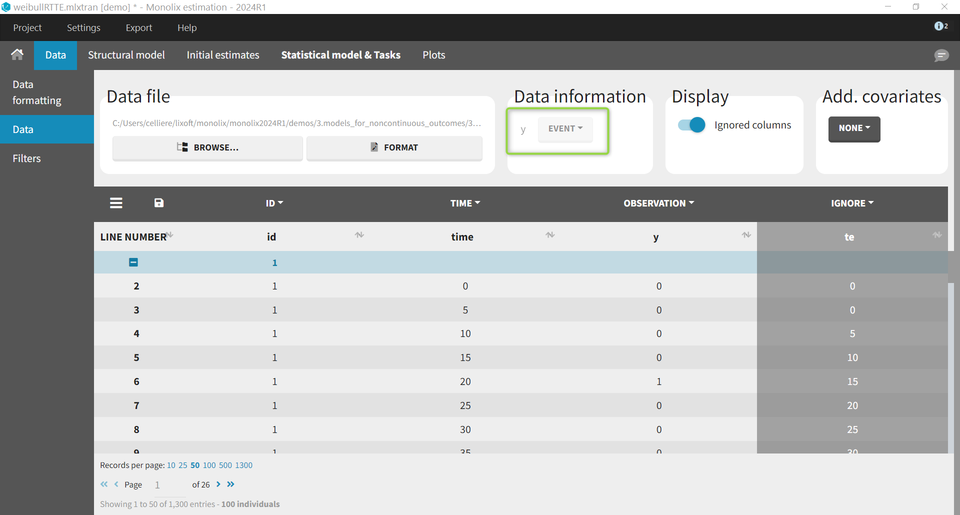
We first show an example where the data is considered as interval-censored repeated time-to-event. After loading the data, the data is indicated as being “EVENT”:

We use a Weibull model with the following hazard, with the shape parameter and the scale parameter:

Its implementation in mlxtran is the following. Note that the interval censoring is indicated using eventType=intervalCensored. The argument intervalLength=5 is optional and is used only for simulations (e.g in the VPC).

[LONGITUDINAL]
input = {lambda, beta}  

EQUATION: 
h = (beta/lambda)*(t/lambda)^(beta-1)

DEFINITION:
Event = {type=event, hazard=h, eventType=intervalCensored,
         intervalLength=5}

OUTPUT:
output = Event

Regarding the statistical model, we keep random effects on both the location and shape parameter as we have several events per individuals which allow to distinguish the inter-individual variability from the randomness of the event time.

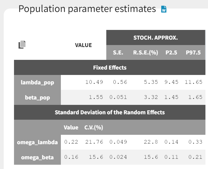
The estimated parameters are shown below. The estimated likelihood is 3552.

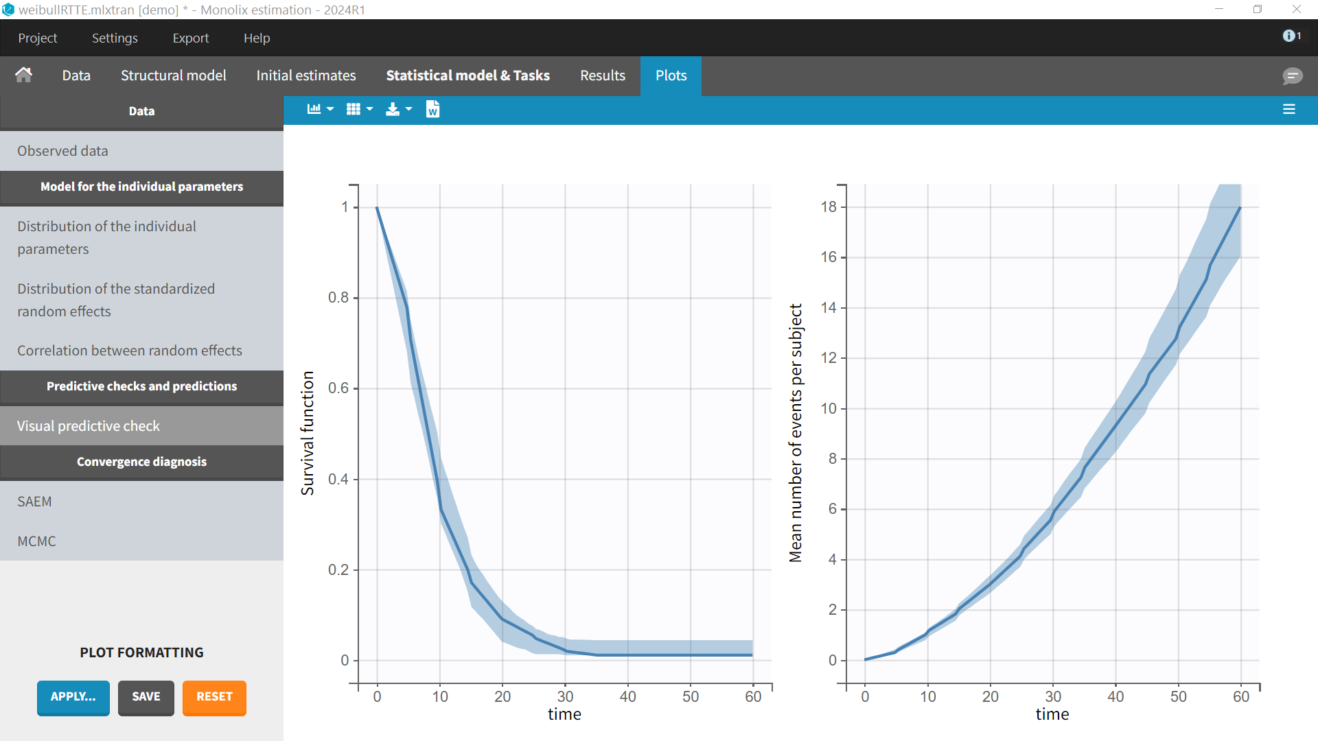
In the diagnostic plots, we can see the Kaplan-Meier curve and corresponding VPC for the first event (left plot) and the mean number of events per subjects (right plot).

• weibullCount (data = weibull_data.txt , model=weibullCount_model.txt)

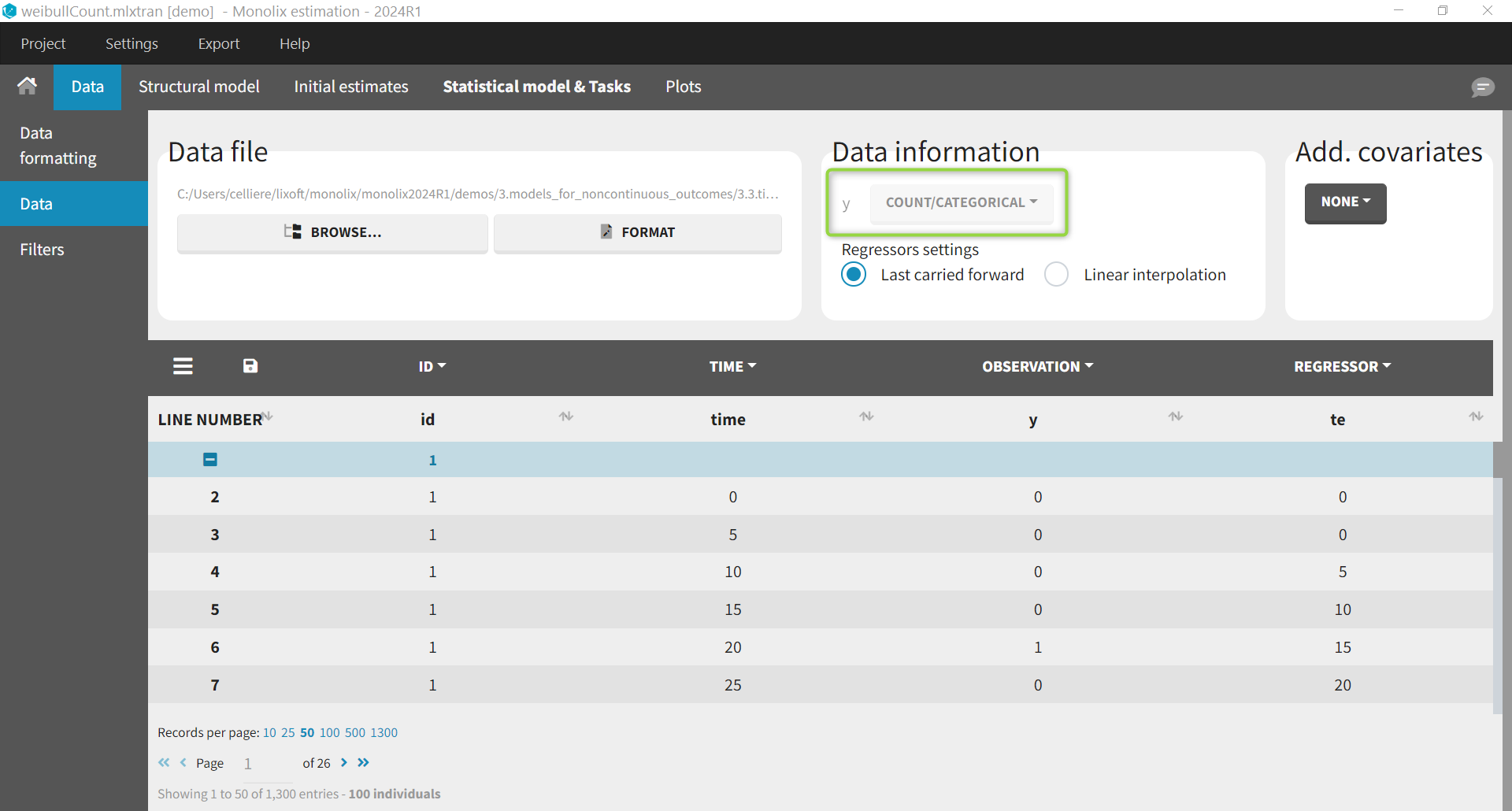
For the same dataset, instead of defining the data as events, it is possible to consider the data as count data: indeed, we count the number of events per interval. After loading the dataset, we indicate the data as being “COUNT/CATEGORICAL”.

To define the model, we start from the the hazard . We then need to obtain the cumulative hazard. For the Weibull model, the hazard integrates into the cumulative hazard as:

To calculate the cumulative hazard in the mlxtran model, we will by pass as REGRESSOR (called tpe in the example below) and obtain the time , which is the current time, using the mlxtran keyword t. Thus, an additional column with the start of the interval is added in the data file and defined as a REGRESSOR.

[LONGITUDINAL]
input = {lambda, beta, tpe}  
tpe = {use=regressor}

EQUATION:
H = (t/lambda)^beta - (tpe/lambda)^beta

The probability to observe events is then defined using the usual formula for Poisson models. We directly define the of the probability, and use an if/else statement to distinguish the case and .

DEFINITION:
nbEvents = {type=count,
if k>0
  lpk = - H + k*log(H) - factln(k)
else
  lpk = - H
end
log(P(Event=k)) = lpk
}

OUTPUT:
output = nbEvents

Note that the count model uses the same parameters as the TTE model: lambda and beta. As for the TTE case, we keep random effects on these two parameters.

The estimated parameters (shown below) are very similar to those estimated with the TTE model.

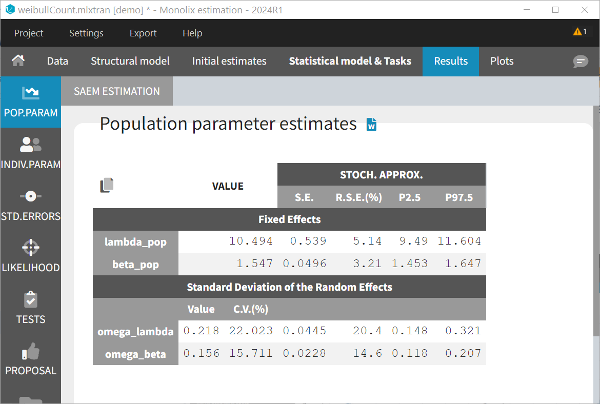
The likelihood is identical (up to 4 digits): 3552.

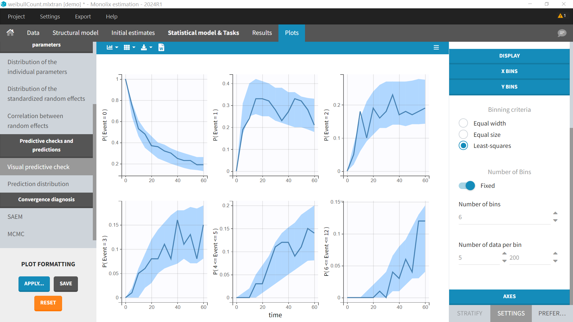
In the diagnostic plots, the VPC shows several subplots corresponding to the probabilities to observe k events (e.g P(Event=0) ), or between k1 and k2 events (e.g P(6<=Event<=12)). The number of subplots can be chosen in the settings “Y Bins”.