Purpose
The log-likelihood is the objective function and a key information. The log-likelihood cannot be computed in closed form for nonlinear mixed effects models. It can however be estimated.
Log-likelihood estimation
Performing likelihood ratio tests and computing information criteria for a given model requires computation of the log-likelihood
where
is the vector of population parameter estimates for the model being considered, and
is the probability distribution function of the observed data given the population parameter estimates. The log-likelihood cannot be computed in closed form for nonlinear mixed effects models. It can however be estimated in a general framework for all kinds of data and models using the importance sampling Monte Carlo method. This method has the advantage of providing an unbiased estimate of the log-likelihood – even for nonlinear models – whose variance can be controlled by the Monte Carlo size.
Two different algorithms are proposed to estimate the log-likelihood:
-
by linearization,
-
by Importance sampling.
Log-likelihood by importance sampling
The observed log-likelihood
can be estimated without requiring approximation of the model, using a Monte Carlo approach. Since
we can estimate
for any individual
. Using the ϕ-representation of the model (the individual parameters are transformed to be Gaussian), notice first that
can be decomposed as follows:
Thus,
is expressed as a mean. It can therefore be approximated by an empirical mean using a Monte Carlo procedure:
-
Draw M independent values
,
, …,
from the marginal distribution
.
-
Estimate
with
.
By construction, this estimator is unbiased, and consistent since its variance decreases as 1/M:
'%3e%3cg transform='translate(167%2c0)'%3e%3cg transform='translate(-13%2c0)'%3e%3cg transform='translate(0%2c-79)'%3e%3cuse xlink:href='%23MJAMS-45' x='0' y='0'%3e%3c/use%3e%3cg transform='translate(834%2c0)'%3e%3cuse xlink:href='%23MJSZ1-28'%3e%3c/use%3e%3cg transform='translate(458%2c0)'%3e%3cuse xlink:href='%23MJMATHI-70' x='0' y='0'%3e%3c/use%3e%3cuse xlink:href='%23MJMAIN-5E' x='84' y='6'%3e%3c/use%3e%3cg transform='translate(585%2c-231)'%3e%3cuse transform='scale(0.707)' xlink:href='%23MJMATHI-69' x='0' y='0'%3e%3c/use%3e%3cuse transform='scale(0.707)' xlink:href='%23MJMAIN-2C' x='345' y='0'%3e%3c/use%3e%3cuse transform='scale(0.707)' xlink:href='%23MJMATHI-4D' x='624' y='0'%3e%3c/use%3e%3c/g%3e%3c/g%3e%3cuse xlink:href='%23MJSZ1-29' x='2328' y='-1'%3e%3c/use%3e%3c/g%3e%3cuse xlink:href='%23MJMAIN-3D' x='3899' y='0'%3e%3c/use%3e%3cg transform='translate(4955%2c0)'%3e%3cuse xlink:href='%23MJAMS-45' x='0' y='0'%3e%3c/use%3e%3cg transform='translate(667%2c-150)'%3e%3cuse transform='scale(0.707)' xlink:href='%23MJMATHI-70' x='0' y='0'%3e%3c/use%3e%3cg transform='translate(356%2c-163)'%3e%3cuse transform='scale(0.5)' xlink:href='%23MJMATHI-3D5' x='0' y='0'%3e%3c/use%3e%3cuse transform='scale(0.5)' xlink:href='%23MJMATHI-69' x='596' y='-318'%3e%3c/use%3e%3c/g%3e%3c/g%3e%3c/g%3e%3cg transform='translate(6837%2c0)'%3e%3cuse xlink:href='%23MJSZ2-28'%3e%3c/use%3e%3cuse xlink:href='%23MJMATHI-70' x='597' y='0'%3e%3c/use%3e%3cuse xlink:href='%23MJMAIN-28' x='1101' y='0'%3e%3c/use%3e%3cg transform='translate(1490%2c0)'%3e%3cuse xlink:href='%23MJMATHI-79' x='0' y='0'%3e%3c/use%3e%3cuse transform='scale(0.707)' xlink:href='%23MJMATHI-69' x='693' y='-213'%3e%3c/use%3e%3c/g%3e%3cuse xlink:href='%23MJMAIN-7C' x='2325' y='0'%3e%3c/use%3e%3cg transform='translate(2603%2c0)'%3e%3cuse xlink:href='%23MJMATHI-3D5' x='0' y='0'%3e%3c/use%3e%3cg transform='translate(596%2c521)'%3e%3cuse transform='scale(0.707)' xlink:href='%23MJMAIN-28' x='0' y='0'%3e%3c/use%3e%3cuse transform='scale(0.707)' xlink:href='%23MJMATHI-6D' x='389' y='0'%3e%3c/use%3e%3cuse transform='scale(0.707)' xlink:href='%23MJMAIN-29' x='1268' y='0'%3e%3c/use%3e%3c/g%3e%3cuse transform='scale(0.707)' xlink:href='%23MJMATHI-69' x='843' y='-430'%3e%3c/use%3e%3c/g%3e%3cuse xlink:href='%23MJMAIN-3B' x='4472' y='0'%3e%3c/use%3e%3cuse xlink:href='%23MJMATHI-3B8' x='4917' y='0'%3e%3c/use%3e%3cuse xlink:href='%23MJMAIN-29' x='5387' y='0'%3e%3c/use%3e%3cuse xlink:href='%23MJSZ2-29' x='5776' y='-1'%3e%3c/use%3e%3c/g%3e%3cuse xlink:href='%23MJMAIN-3D' x='13488' y='0'%3e%3c/use%3e%3cuse xlink:href='%23MJMATHI-70' x='14545' y='0'%3e%3c/use%3e%3cuse xlink:href='%23MJMAIN-28' x='15048' y='0'%3e%3c/use%3e%3cg transform='translate(15438%2c0)'%3e%3cuse xlink:href='%23MJMATHI-79' x='0' y='0'%3e%3c/use%3e%3cuse transform='scale(0.707)' xlink:href='%23MJMATHI-69' x='693' y='-213'%3e%3c/use%3e%3c/g%3e%3cuse xlink:href='%23MJMAIN-3B' x='16273' y='0'%3e%3c/use%3e%3cuse xlink:href='%23MJMATHI-3B8' x='16718' y='0'%3e%3c/use%3e%3cuse xlink:href='%23MJMAIN-29' x='17187' y='0'%3e%3c/use%3e%3cg transform='translate(18577%2c0)'%3e%3cuse xlink:href='%23MJMAIN-56'%3e%3c/use%3e%3cuse xlink:href='%23MJMAIN-61' x='750' y='0'%3e%3c/use%3e%3cuse xlink:href='%23MJMAIN-72' x='1251' y='0'%3e%3c/use%3e%3c/g%3e%3cg transform='translate(20387%2c0)'%3e%3cuse xlink:href='%23MJSZ1-28'%3e%3c/use%3e%3cg transform='translate(458%2c0)'%3e%3cuse xlink:href='%23MJMATHI-70' x='0' y='0'%3e%3c/use%3e%3cuse xlink:href='%23MJMAIN-5E' x='84' y='6'%3e%3c/use%3e%3cg transform='translate(585%2c-231)'%3e%3cuse transform='scale(0.707)' xlink:href='%23MJMATHI-69' x='0' y='0'%3e%3c/use%3e%3cuse transform='scale(0.707)' xlink:href='%23MJMAIN-2C' x='345' y='0'%3e%3c/use%3e%3cuse transform='scale(0.707)' xlink:href='%23MJMATHI-4D' x='624' y='0'%3e%3c/use%3e%3c/g%3e%3c/g%3e%3cuse xlink:href='%23MJSZ1-29' x='2328' y='-1'%3e%3c/use%3e%3c/g%3e%3cuse xlink:href='%23MJMAIN-3D' x='23452' y='0'%3e%3c/use%3e%3cg transform='translate(24230%2c0)'%3e%3cg transform='translate(397%2c0)'%3e%3crect stroke='none' width='1171' height='60' x='0' y='220'%3e%3c/rect%3e%3cuse xlink:href='%23MJMAIN-31' x='335' y='676'%3e%3c/use%3e%3cuse xlink:href='%23MJMATHI-4D' x='60' y='-686'%3e%3c/use%3e%3c/g%3e%3c/g%3e%3cg transform='translate(25919%2c0)'%3e%3cuse xlink:href='%23MJMAIN-56'%3e%3c/use%3e%3cuse xlink:href='%23MJMAIN-61' x='750' y='0'%3e%3c/use%3e%3cuse xlink:href='%23MJMAIN-72' x='1251' y='0'%3e%3c/use%3e%3cg transform='translate(1643%2c-150)'%3e%3cuse transform='scale(0.707)' xlink:href='%23MJMATHI-70' x='0' y='0'%3e%3c/use%3e%3cg transform='translate(356%2c-163)'%3e%3cuse transform='scale(0.5)' xlink:href='%23MJMATHI-3D5' x='0' y='0'%3e%3c/use%3e%3cuse transform='scale(0.5)' xlink:href='%23MJMATHI-69' x='596' y='-318'%3e%3c/use%3e%3c/g%3e%3c/g%3e%3c/g%3e%3cg transform='translate(28777%2c0)'%3e%3cuse xlink:href='%23MJSZ2-28'%3e%3c/use%3e%3cuse xlink:href='%23MJMATHI-70' x='597' y='0'%3e%3c/use%3e%3cuse xlink:href='%23MJMAIN-28' x='1101' y='0'%3e%3c/use%3e%3cg transform='translate(1490%2c0)'%3e%3cuse xlink:href='%23MJMATHI-79' x='0' y='0'%3e%3c/use%3e%3cuse transform='scale(0.707)' xlink:href='%23MJMATHI-69' x='693' y='-213'%3e%3c/use%3e%3c/g%3e%3cuse xlink:href='%23MJMAIN-7C' x='2325' y='0'%3e%3c/use%3e%3cg transform='translate(2603%2c0)'%3e%3cuse xlink:href='%23MJMATHI-3D5' x='0' y='0'%3e%3c/use%3e%3cg transform='translate(596%2c521)'%3e%3cuse transform='scale(0.707)' xlink:href='%23MJMAIN-28' x='0' y='0'%3e%3c/use%3e%3cuse transform='scale(0.707)' xlink:href='%23MJMATHI-6D' x='389' y='0'%3e%3c/use%3e%3cuse transform='scale(0.707)' xlink:href='%23MJMAIN-29' x='1268' y='0'%3e%3c/use%3e%3c/g%3e%3cuse transform='scale(0.707)' xlink:href='%23MJMATHI-69' x='843' y='-430'%3e%3c/use%3e%3c/g%3e%3cuse xlink:href='%23MJMAIN-3B' x='4472' y='0'%3e%3c/use%3e%3cuse xlink:href='%23MJMATHI-3B8' x='4917' y='0'%3e%3c/use%3e%3cuse xlink:href='%23MJMAIN-29' x='5387' y='0'%3e%3c/use%3e%3cuse xlink:href='%23MJSZ2-29' x='5776' y='-1'%3e%3c/use%3e%3c/g%3e%3c/g%3e%3c/g%3e%3c/g%3e%3c/g%3e%3c/svg%3e)
We could consider ourselves satisfied with this estimator since we “only” have to select M large enough to get an estimator with a small variance. Nevertheless, it is possible to improve the statistical properties of this estimator.
For any distribution
'%3e%3cg transform='translate(167%2c0)'%3e%3cg transform='translate(-13%2c0)'%3e%3cg transform='translate(0%2c13)'%3e%3cuse xlink:href='%23MJMATHI-70' x='0' y='0'%3e%3c/use%3e%3cg transform='translate(503%2c-150)'%3e%3cuse transform='scale(0.707)' xlink:href='%23MJMATHI-3D5' x='0' y='0'%3e%3c/use%3e%3cuse transform='scale(0.5)' xlink:href='%23MJMATHI-69' x='843' y='-342'%3e%3c/use%3e%3c/g%3e%3cuse xlink:href='%23MJMAIN-7E' x='384' y='322'%3e%3c/use%3e%3c/g%3e%3c/g%3e%3c/g%3e%3c/g%3e%3c/svg%3e) that is absolutely continuous with respect to the marginal distribution
that is absolutely continuous with respect to the marginal distribution
'%3e%3cg transform='translate(167%2c0)'%3e%3cg transform='translate(-13%2c0)'%3e%3cg transform='translate(0%2c13)'%3e%3cuse xlink:href='%23MJMATHI-70' x='0' y='0'%3e%3c/use%3e%3cg transform='translate(503%2c-150)'%3e%3cuse transform='scale(0.707)' xlink:href='%23MJMATHI-3D5' x='0' y='0'%3e%3c/use%3e%3cuse transform='scale(0.5)' xlink:href='%23MJMATHI-69' x='843' y='-342'%3e%3c/use%3e%3c/g%3e%3c/g%3e%3c/g%3e%3c/g%3e%3c/g%3e%3c/svg%3e) , we can write
, we can write
We can now approximate
'%3e%3cg transform='translate(167%2c0)'%3e%3cg transform='translate(-13%2c0)'%3e%3cg transform='translate(0%2c-25)'%3e%3cuse xlink:href='%23MJMATHI-70' x='0' y='0'%3e%3c/use%3e%3cuse xlink:href='%23MJMAIN-28' x='503' y='0'%3e%3c/use%3e%3cg transform='translate(893%2c0)'%3e%3cuse xlink:href='%23MJMATHI-79' x='0' y='0'%3e%3c/use%3e%3cuse transform='scale(0.707)' xlink:href='%23MJMATHI-69' x='693' y='-213'%3e%3c/use%3e%3c/g%3e%3cuse xlink:href='%23MJMAIN-3B' x='1727' y='0'%3e%3c/use%3e%3cuse xlink:href='%23MJMATHI-3B8' x='2172' y='0'%3e%3c/use%3e%3cuse xlink:href='%23MJMAIN-29' x='2642' y='0'%3e%3c/use%3e%3c/g%3e%3c/g%3e%3c/g%3e%3c/g%3e%3c/svg%3e) using an importance sampling integration method with
as the proposal distribution:
using an importance sampling integration method with
as the proposal distribution:
-
Draw M independent values
![]() ,
,
![]() , …,
, …,
![]() from the marginal distribution
from the marginal distribution
![]() .
. -
Estimate
![]() with
with
.
'%3e%3cg transform='translate(167%2c0)'%3e%3cg transform='translate(-13%2c0)'%3e%3cg transform='translate(0%2c-121)'%3e%3cuse xlink:href='%23MJMATHI-3D5' x='0' y='0'%3e%3c/use%3e%3cg transform='translate(596%2c521)'%3e%3cuse transform='scale(0.707)' xlink:href='%23MJMAIN-28' x='0' y='0'%3e%3c/use%3e%3cuse transform='scale(0.707)' xlink:href='%23MJMAIN-31' x='389' y='0'%3e%3c/use%3e%3cuse transform='scale(0.707)' xlink:href='%23MJMAIN-29' x='890' y='0'%3e%3c/use%3e%3c/g%3e%3cuse transform='scale(0.707)' xlink:href='%23MJMATHI-69' x='843' y='-430'%3e%3c/use%3e%3c/g%3e%3c/g%3e%3c/g%3e%3c/g%3e%3c/svg%3e)
'%3e%3cg transform='translate(167%2c0)'%3e%3cg transform='translate(-13%2c0)'%3e%3cg transform='translate(0%2c-121)'%3e%3cuse xlink:href='%23MJMATHI-3D5' x='0' y='0'%3e%3c/use%3e%3cg transform='translate(596%2c521)'%3e%3cuse transform='scale(0.707)' xlink:href='%23MJMAIN-28' x='0' y='0'%3e%3c/use%3e%3cuse transform='scale(0.707)' xlink:href='%23MJMAIN-32' x='389' y='0'%3e%3c/use%3e%3cuse transform='scale(0.707)' xlink:href='%23MJMAIN-29' x='890' y='0'%3e%3c/use%3e%3c/g%3e%3cuse transform='scale(0.707)' xlink:href='%23MJMATHI-69' x='843' y='-430'%3e%3c/use%3e%3c/g%3e%3c/g%3e%3c/g%3e%3c/g%3e%3c/svg%3e)
'%3e%3cg transform='translate(167%2c0)'%3e%3cg transform='translate(-13%2c0)'%3e%3cg transform='translate(0%2c-121)'%3e%3cuse xlink:href='%23MJMATHI-3D5' x='0' y='0'%3e%3c/use%3e%3cg transform='translate(596%2c521)'%3e%3cuse transform='scale(0.707)' xlink:href='%23MJMAIN-28' x='0' y='0'%3e%3c/use%3e%3cuse transform='scale(0.707)' xlink:href='%23MJMATHI-4D' x='389' y='0'%3e%3c/use%3e%3cuse transform='scale(0.707)' xlink:href='%23MJMAIN-29' x='1441' y='0'%3e%3c/use%3e%3c/g%3e%3cuse transform='scale(0.707)' xlink:href='%23MJMATHI-69' x='843' y='-430'%3e%3c/use%3e%3c/g%3e%3c/g%3e%3c/g%3e%3c/g%3e%3c/svg%3e)
'%3e%3cg transform='translate(167%2c0)'%3e%3cg transform='translate(-13%2c0)'%3e%3cg transform='translate(0%2c13)'%3e%3cuse xlink:href='%23MJMATHI-70' x='0' y='0'%3e%3c/use%3e%3cg transform='translate(503%2c-150)'%3e%3cuse transform='scale(0.707)' xlink:href='%23MJMATHI-3D5' x='0' y='0'%3e%3c/use%3e%3cuse transform='scale(0.5)' xlink:href='%23MJMATHI-69' x='843' y='-342'%3e%3c/use%3e%3c/g%3e%3cuse xlink:href='%23MJMAIN-28' x='1268' y='0'%3e%3c/use%3e%3cuse xlink:href='%23MJMAIN-2E' x='1658' y='0'%3e%3c/use%3e%3cuse xlink:href='%23MJMAIN-3B' x='2103' y='0'%3e%3c/use%3e%3cuse xlink:href='%23MJMATHI-3B8' x='2548' y='0'%3e%3c/use%3e%3cuse xlink:href='%23MJMAIN-29' x='3018' y='0'%3e%3c/use%3e%3c/g%3e%3c/g%3e%3c/g%3e%3c/g%3e%3c/svg%3e)
'%3e%3cg transform='translate(167%2c0)'%3e%3cg transform='translate(-13%2c0)'%3e%3cg transform='translate(0%2c-25)'%3e%3cuse xlink:href='%23MJMAIN-6C'%3e%3c/use%3e%3cuse xlink:href='%23MJMAIN-6F' x='278' y='0'%3e%3c/use%3e%3cuse xlink:href='%23MJMAIN-67' x='779' y='0'%3e%3c/use%3e%3cuse xlink:href='%23MJMAIN-28' x='1279' y='0'%3e%3c/use%3e%3cuse xlink:href='%23MJMATHI-70' x='1669' y='0'%3e%3c/use%3e%3cuse xlink:href='%23MJMAIN-28' x='2172' y='0'%3e%3c/use%3e%3cg transform='translate(2562%2c0)'%3e%3cuse xlink:href='%23MJMATHI-79' x='0' y='0'%3e%3c/use%3e%3cuse transform='scale(0.707)' xlink:href='%23MJMATHI-69' x='693' y='-213'%3e%3c/use%3e%3c/g%3e%3cuse xlink:href='%23MJMAIN-3B' x='3396' y='0'%3e%3c/use%3e%3cuse xlink:href='%23MJMATHI-3B8' x='3841' y='0'%3e%3c/use%3e%3cuse xlink:href='%23MJMAIN-29' x='4311' y='0'%3e%3c/use%3e%3cuse xlink:href='%23MJMAIN-29' x='4700' y='0'%3e%3c/use%3e%3c/g%3e%3c/g%3e%3c/g%3e%3c/g%3e%3c/svg%3e)
By construction, this estimator is unbiased, and its variance also decreases as 1/M:
'%3e%3cg transform='translate(167%2c0)'%3e%3cg transform='translate(-13%2c0)'%3e%3cuse xlink:href='%23MJMAIN-56'%3e%3c/use%3e%3cuse xlink:href='%23MJMAIN-61' x='750' y='0'%3e%3c/use%3e%3cuse xlink:href='%23MJMAIN-72' x='1251' y='0'%3e%3c/use%3e%3cg transform='translate(1810%2c0)'%3e%3cuse xlink:href='%23MJSZ1-28'%3e%3c/use%3e%3cg transform='translate(458%2c0)'%3e%3cuse xlink:href='%23MJMATHI-70' x='0' y='0'%3e%3c/use%3e%3cuse xlink:href='%23MJMAIN-5E' x='84' y='6'%3e%3c/use%3e%3cg transform='translate(585%2c-231)'%3e%3cuse transform='scale(0.707)' xlink:href='%23MJMATHI-69' x='0' y='0'%3e%3c/use%3e%3cuse transform='scale(0.707)' xlink:href='%23MJMAIN-2C' x='345' y='0'%3e%3c/use%3e%3cuse transform='scale(0.707)' xlink:href='%23MJMATHI-4D' x='624' y='0'%3e%3c/use%3e%3c/g%3e%3c/g%3e%3cuse xlink:href='%23MJSZ1-29' x='2328' y='-1'%3e%3c/use%3e%3c/g%3e%3cuse xlink:href='%23MJMAIN-3D' x='4875' y='0'%3e%3c/use%3e%3cg transform='translate(5653%2c0)'%3e%3cg transform='translate(397%2c0)'%3e%3crect stroke='none' width='1171' height='60' x='0' y='220'%3e%3c/rect%3e%3cuse xlink:href='%23MJMAIN-31' x='335' y='676'%3e%3c/use%3e%3cuse xlink:href='%23MJMATHI-4D' x='60' y='-686'%3e%3c/use%3e%3c/g%3e%3c/g%3e%3cg transform='translate(7342%2c0)'%3e%3cuse xlink:href='%23MJMAIN-56'%3e%3c/use%3e%3cuse xlink:href='%23MJMAIN-61' x='750' y='0'%3e%3c/use%3e%3cuse xlink:href='%23MJMAIN-72' x='1251' y='0'%3e%3c/use%3e%3cg transform='translate(1643%2c-150)'%3e%3cuse transform='scale(0.707)' xlink:href='%23MJMATHI-70' x='0' y='0'%3e%3c/use%3e%3cg transform='translate(356%2c-163)'%3e%3cuse transform='scale(0.5)' xlink:href='%23MJMATHI-3D5' x='0' y='0'%3e%3c/use%3e%3cuse transform='scale(0.5)' xlink:href='%23MJMATHI-69' x='596' y='-318'%3e%3c/use%3e%3c/g%3e%3cuse transform='scale(0.707)' xlink:href='%23MJMAIN-7E' x='419' y='360'%3e%3c/use%3e%3c/g%3e%3c/g%3e%3cg transform='translate(10200%2c0)'%3e%3cuse xlink:href='%23MJSZ4-28'%3e%3c/use%3e%3cuse xlink:href='%23MJMATHI-70' x='792' y='0'%3e%3c/use%3e%3cuse xlink:href='%23MJMAIN-28' x='1296' y='0'%3e%3c/use%3e%3cg transform='translate(1685%2c0)'%3e%3cuse xlink:href='%23MJMATHI-79' x='0' y='0'%3e%3c/use%3e%3cuse transform='scale(0.707)' xlink:href='%23MJMATHI-69' x='693' y='-213'%3e%3c/use%3e%3c/g%3e%3cuse xlink:href='%23MJMAIN-7C' x='2520' y='0'%3e%3c/use%3e%3cg transform='translate(2798%2c0)'%3e%3cuse xlink:href='%23MJMATHI-3D5' x='0' y='0'%3e%3c/use%3e%3cg transform='translate(596%2c521)'%3e%3cuse transform='scale(0.707)' xlink:href='%23MJMAIN-28' x='0' y='0'%3e%3c/use%3e%3cuse transform='scale(0.707)' xlink:href='%23MJMATHI-6D' x='389' y='0'%3e%3c/use%3e%3cuse transform='scale(0.707)' xlink:href='%23MJMAIN-29' x='1268' y='0'%3e%3c/use%3e%3c/g%3e%3cuse transform='scale(0.707)' xlink:href='%23MJMATHI-69' x='843' y='-430'%3e%3c/use%3e%3c/g%3e%3cuse xlink:href='%23MJMAIN-3B' x='4667' y='0'%3e%3c/use%3e%3cuse xlink:href='%23MJMATHI-3B8' x='5112' y='0'%3e%3c/use%3e%3cuse xlink:href='%23MJMAIN-29' x='5582' y='0'%3e%3c/use%3e%3cg transform='translate(5971%2c0)'%3e%3cg transform='translate(120%2c0)'%3e%3crect stroke='none' width='4267' height='60' x='0' y='220'%3e%3c/rect%3e%3cg transform='translate(100%2c805)'%3e%3cuse xlink:href='%23MJMATHI-70' x='0' y='0'%3e%3c/use%3e%3cuse xlink:href='%23MJMAIN-28' x='503' y='0'%3e%3c/use%3e%3cg transform='translate(893%2c0)'%3e%3cuse xlink:href='%23MJMATHI-3D5' x='0' y='0'%3e%3c/use%3e%3cg transform='translate(596%2c521)'%3e%3cuse transform='scale(0.707)' xlink:href='%23MJMAIN-28' x='0' y='0'%3e%3c/use%3e%3cuse transform='scale(0.707)' xlink:href='%23MJMATHI-6D' x='389' y='0'%3e%3c/use%3e%3cuse transform='scale(0.707)' xlink:href='%23MJMAIN-29' x='1268' y='0'%3e%3c/use%3e%3c/g%3e%3cuse transform='scale(0.707)' xlink:href='%23MJMATHI-69' x='843' y='-430'%3e%3c/use%3e%3c/g%3e%3cuse xlink:href='%23MJMAIN-3B' x='2761' y='0'%3e%3c/use%3e%3cuse xlink:href='%23MJMATHI-3B8' x='3206' y='0'%3e%3c/use%3e%3cuse xlink:href='%23MJMAIN-29' x='3676' y='0'%3e%3c/use%3e%3c/g%3e%3cg transform='translate(60%2c-1047)'%3e%3cuse xlink:href='%23MJMATHI-70' x='0' y='0'%3e%3c/use%3e%3cuse xlink:href='%23MJMAIN-7E' x='84' y='322'%3e%3c/use%3e%3cuse xlink:href='%23MJMAIN-28' x='585' y='0'%3e%3c/use%3e%3cg transform='translate(974%2c0)'%3e%3cuse xlink:href='%23MJMATHI-3D5' x='0' y='0'%3e%3c/use%3e%3cg transform='translate(596%2c521)'%3e%3cuse transform='scale(0.707)' xlink:href='%23MJMAIN-28' x='0' y='0'%3e%3c/use%3e%3cuse transform='scale(0.707)' xlink:href='%23MJMATHI-6D' x='389' y='0'%3e%3c/use%3e%3cuse transform='scale(0.707)' xlink:href='%23MJMAIN-29' x='1268' y='0'%3e%3c/use%3e%3c/g%3e%3cuse transform='scale(0.707)' xlink:href='%23MJMATHI-69' x='843' y='-430'%3e%3c/use%3e%3c/g%3e%3cuse xlink:href='%23MJMAIN-3B' x='2843' y='0'%3e%3c/use%3e%3cuse xlink:href='%23MJMATHI-3B8' x='3288' y='0'%3e%3c/use%3e%3cuse xlink:href='%23MJMAIN-29' x='3757' y='0'%3e%3c/use%3e%3c/g%3e%3c/g%3e%3c/g%3e%3cuse xlink:href='%23MJSZ4-29' x='10478' y='0'%3e%3c/use%3e%3c/g%3e%3c/g%3e%3c/g%3e%3c/g%3e%3c/svg%3e)
There exist an infinite number of possible proposal distributions
'%3e%3cg transform='translate(167%2c0)'%3e%3cg transform='translate(-13%2c0)'%3e%3cg transform='translate(0%2c-50)'%3e%3cuse xlink:href='%23MJMATHI-70' x='0' y='0'%3e%3c/use%3e%3cuse xlink:href='%23MJMAIN-7E' x='84' y='322'%3e%3c/use%3e%3c/g%3e%3c/g%3e%3c/g%3e%3c/g%3e%3c/svg%3e) which all provide the same rate of convergence 1/M. The trick is to reduce the variance of the estimator by selecting a proposal distribution so that the numerator is as small as possible.
which all provide the same rate of convergence 1/M. The trick is to reduce the variance of the estimator by selecting a proposal distribution so that the numerator is as small as possible.
For this purpose, an optimal proposal distribution would be the conditional distribution
'%3e%3cg transform='translate(167%2c0)'%3e%3cg transform='translate(-13%2c0)'%3e%3cg transform='translate(0%2c31)'%3e%3cuse xlink:href='%23MJMATHI-70' x='0' y='0'%3e%3c/use%3e%3cg transform='translate(503%2c-187)'%3e%3cuse transform='scale(0.707)' xlink:href='%23MJMATHI-3D5' x='0' y='0'%3e%3c/use%3e%3cuse transform='scale(0.5)' xlink:href='%23MJMATHI-69' x='843' y='-342'%3e%3c/use%3e%3cuse transform='scale(0.707)' xlink:href='%23MJMAIN-7C' x='940' y='0'%3e%3c/use%3e%3cg transform='translate(862%2c0)'%3e%3cuse transform='scale(0.707)' xlink:href='%23MJMATHI-79' x='0' y='0'%3e%3c/use%3e%3cuse transform='scale(0.5)' xlink:href='%23MJMATHI-69' x='693' y='-342'%3e%3c/use%3e%3c/g%3e%3c/g%3e%3c/g%3e%3c/g%3e%3c/g%3e%3c/g%3e%3c/svg%3e) . Indeed, for any
. Indeed, for any
'%3e%3cg transform='translate(167%2c0)'%3e%3cg transform='translate(-13%2c0)'%3e%3cg transform='translate(0%2c-50)'%3e%3cuse xlink:href='%23MJMATHI-6D' x='0' y='0'%3e%3c/use%3e%3cuse xlink:href='%23MJMAIN-3D' x='1156' y='0'%3e%3c/use%3e%3cuse xlink:href='%23MJMAIN-31' x='2212' y='0'%3e%3c/use%3e%3cuse xlink:href='%23MJMAIN-2C' x='2713' y='0'%3e%3c/use%3e%3cuse xlink:href='%23MJMAIN-32' x='3158' y='0'%3e%3c/use%3e%3cuse xlink:href='%23MJMAIN-2C' x='3658' y='0'%3e%3c/use%3e%3cuse xlink:href='%23MJMAIN-2E' x='4103' y='0'%3e%3c/use%3e%3cuse xlink:href='%23MJMAIN-2E' x='4549' y='0'%3e%3c/use%3e%3cuse xlink:href='%23MJMAIN-2E' x='4994' y='0'%3e%3c/use%3e%3cuse xlink:href='%23MJMAIN-2C' x='5439' y='0'%3e%3c/use%3e%3cuse xlink:href='%23MJMATHI-4D' x='5884' y='0'%3e%3c/use%3e%3c/g%3e%3c/g%3e%3c/g%3e%3c/g%3e%3c/svg%3e) ,
,
'%3e%3cg transform='translate(167%2c0)'%3e%3cg transform='translate(-13%2c0)'%3e%3cuse xlink:href='%23MJMATHI-70' x='0' y='0'%3e%3c/use%3e%3cuse xlink:href='%23MJMAIN-28' x='503' y='0'%3e%3c/use%3e%3cg transform='translate(893%2c0)'%3e%3cuse xlink:href='%23MJMATHI-79' x='0' y='0'%3e%3c/use%3e%3cuse transform='scale(0.707)' xlink:href='%23MJMATHI-69' x='693' y='-213'%3e%3c/use%3e%3c/g%3e%3cuse xlink:href='%23MJMAIN-7C' x='1727' y='0'%3e%3c/use%3e%3cg transform='translate(2006%2c0)'%3e%3cuse xlink:href='%23MJMATHI-3D5' x='0' y='0'%3e%3c/use%3e%3cg transform='translate(596%2c521)'%3e%3cuse transform='scale(0.707)' xlink:href='%23MJMAIN-28' x='0' y='0'%3e%3c/use%3e%3cuse transform='scale(0.707)' xlink:href='%23MJMATHI-6D' x='389' y='0'%3e%3c/use%3e%3cuse transform='scale(0.707)' xlink:href='%23MJMAIN-29' x='1268' y='0'%3e%3c/use%3e%3c/g%3e%3cuse transform='scale(0.707)' xlink:href='%23MJMATHI-69' x='843' y='-430'%3e%3c/use%3e%3c/g%3e%3cuse xlink:href='%23MJMAIN-3B' x='3874' y='0'%3e%3c/use%3e%3cuse xlink:href='%23MJMATHI-3B8' x='4320' y='0'%3e%3c/use%3e%3cuse xlink:href='%23MJMAIN-29' x='4789' y='0'%3e%3c/use%3e%3cg transform='translate(5179%2c0)'%3e%3cg transform='translate(120%2c0)'%3e%3crect stroke='none' width='5299' height='60' x='0' y='220'%3e%3c/rect%3e%3cg transform='translate(616%2c805)'%3e%3cuse xlink:href='%23MJMATHI-70' x='0' y='0'%3e%3c/use%3e%3cuse xlink:href='%23MJMAIN-28' x='503' y='0'%3e%3c/use%3e%3cg transform='translate(893%2c0)'%3e%3cuse xlink:href='%23MJMATHI-3D5' x='0' y='0'%3e%3c/use%3e%3cg transform='translate(596%2c521)'%3e%3cuse transform='scale(0.707)' xlink:href='%23MJMAIN-28' x='0' y='0'%3e%3c/use%3e%3cuse transform='scale(0.707)' xlink:href='%23MJMATHI-6D' x='389' y='0'%3e%3c/use%3e%3cuse transform='scale(0.707)' xlink:href='%23MJMAIN-29' x='1268' y='0'%3e%3c/use%3e%3c/g%3e%3cuse transform='scale(0.707)' xlink:href='%23MJMATHI-69' x='843' y='-430'%3e%3c/use%3e%3c/g%3e%3cuse xlink:href='%23MJMAIN-3B' x='2761' y='0'%3e%3c/use%3e%3cuse xlink:href='%23MJMATHI-3B8' x='3206' y='0'%3e%3c/use%3e%3cuse xlink:href='%23MJMAIN-29' x='3676' y='0'%3e%3c/use%3e%3c/g%3e%3cg transform='translate(60%2c-1047)'%3e%3cuse xlink:href='%23MJMATHI-70' x='0' y='0'%3e%3c/use%3e%3cuse xlink:href='%23MJMAIN-28' x='503' y='0'%3e%3c/use%3e%3cg transform='translate(893%2c0)'%3e%3cuse xlink:href='%23MJMATHI-3D5' x='0' y='0'%3e%3c/use%3e%3cg transform='translate(596%2c521)'%3e%3cuse transform='scale(0.707)' xlink:href='%23MJMAIN-28' x='0' y='0'%3e%3c/use%3e%3cuse transform='scale(0.707)' xlink:href='%23MJMATHI-6D' x='389' y='0'%3e%3c/use%3e%3cuse transform='scale(0.707)' xlink:href='%23MJMAIN-29' x='1268' y='0'%3e%3c/use%3e%3c/g%3e%3cuse transform='scale(0.707)' xlink:href='%23MJMATHI-69' x='843' y='-430'%3e%3c/use%3e%3c/g%3e%3cuse xlink:href='%23MJMAIN-7C' x='2761' y='0'%3e%3c/use%3e%3cg transform='translate(3040%2c0)'%3e%3cuse xlink:href='%23MJMATHI-79' x='0' y='0'%3e%3c/use%3e%3cuse transform='scale(0.707)' xlink:href='%23MJMATHI-69' x='693' y='-213'%3e%3c/use%3e%3c/g%3e%3cuse xlink:href='%23MJMAIN-3B' x='3874' y='0'%3e%3c/use%3e%3cuse xlink:href='%23MJMATHI-3B8' x='4320' y='0'%3e%3c/use%3e%3cuse xlink:href='%23MJMAIN-29' x='4789' y='0'%3e%3c/use%3e%3c/g%3e%3c/g%3e%3c/g%3e%3cuse xlink:href='%23MJMAIN-3D' x='10995' y='0'%3e%3c/use%3e%3cuse xlink:href='%23MJMATHI-70' x='12052' y='0'%3e%3c/use%3e%3cuse xlink:href='%23MJMAIN-28' x='12555' y='0'%3e%3c/use%3e%3cg transform='translate(12945%2c0)'%3e%3cuse xlink:href='%23MJMATHI-79' x='0' y='0'%3e%3c/use%3e%3cuse transform='scale(0.707)' xlink:href='%23MJMATHI-69' x='693' y='-213'%3e%3c/use%3e%3c/g%3e%3cuse xlink:href='%23MJMAIN-3B' x='13779' y='0'%3e%3c/use%3e%3cuse xlink:href='%23MJMATHI-3B8' x='14225' y='0'%3e%3c/use%3e%3cuse xlink:href='%23MJMAIN-29' x='14694' y='0'%3e%3c/use%3e%3c/g%3e%3c/g%3e%3c/g%3e%3c/svg%3e)
which has a zero variance, so that only one draw from
is required to exactly compute the likelihood
.
The problem is that it is not possible to generate the
'%3e%3cg transform='translate(167%2c0)'%3e%3cg transform='translate(-13%2c0)'%3e%3cg transform='translate(0%2c-121)'%3e%3cuse xlink:href='%23MJMATHI-3D5' x='0' y='0'%3e%3c/use%3e%3cg transform='translate(596%2c521)'%3e%3cuse transform='scale(0.707)' xlink:href='%23MJMAIN-28' x='0' y='0'%3e%3c/use%3e%3cuse transform='scale(0.707)' xlink:href='%23MJMATHI-6D' x='389' y='0'%3e%3c/use%3e%3cuse transform='scale(0.707)' xlink:href='%23MJMAIN-29' x='1268' y='0'%3e%3c/use%3e%3c/g%3e%3cuse transform='scale(0.707)' xlink:href='%23MJMATHI-69' x='843' y='-430'%3e%3c/use%3e%3c/g%3e%3c/g%3e%3c/g%3e%3c/g%3e%3c/svg%3e) with this exact conditional distribution, since that would require computing a normalizing constant, which here is precisely
with this exact conditional distribution, since that would require computing a normalizing constant, which here is precisely
.
Nevertheless, this conditional distribution can be estimated using the Metropolis-Hastings algorithm and a practical proposal “close” to the optimal proposal
can be derived. We can then expect to get a very accurate estimate with a relatively small Monte Carlo size M.
The mean and variance of the conditional distribution
are estimated by Metropolis-Hastings for each individual
. Then, the
are drawn with a non-central student t-distribution:
'%3e%3cg transform='translate(167%2c0)'%3e%3cg transform='translate(-13%2c0)'%3e%3cg transform='translate(0%2c-121)'%3e%3cuse xlink:href='%23MJMATHI-3D5' x='0' y='0'%3e%3c/use%3e%3cg transform='translate(596%2c521)'%3e%3cuse transform='scale(0.707)' xlink:href='%23MJMAIN-28' x='0' y='0'%3e%3c/use%3e%3cuse transform='scale(0.707)' xlink:href='%23MJMATHI-6D' x='389' y='0'%3e%3c/use%3e%3cuse transform='scale(0.707)' xlink:href='%23MJMAIN-29' x='1268' y='0'%3e%3c/use%3e%3c/g%3e%3cuse transform='scale(0.707)' xlink:href='%23MJMATHI-69' x='843' y='-430'%3e%3c/use%3e%3cuse xlink:href='%23MJMAIN-3D' x='2146' y='0'%3e%3c/use%3e%3cg transform='translate(3202%2c0)'%3e%3cuse xlink:href='%23MJMATHI-3BC' x='0' y='0'%3e%3c/use%3e%3cuse transform='scale(0.707)' xlink:href='%23MJMATHI-69' x='853' y='-213'%3e%3c/use%3e%3c/g%3e%3cuse xlink:href='%23MJMAIN-2B' x='4372' y='0'%3e%3c/use%3e%3cg transform='translate(5373%2c0)'%3e%3cuse xlink:href='%23MJMATHI-3C3' x='0' y='0'%3e%3c/use%3e%3cuse transform='scale(0.707)' xlink:href='%23MJMATHI-69' x='808' y='-213'%3e%3c/use%3e%3c/g%3e%3cuse xlink:href='%23MJMAIN-D7' x='6511' y='0'%3e%3c/use%3e%3cg transform='translate(7512%2c0)'%3e%3cuse xlink:href='%23MJMATHI-54' x='0' y='0'%3e%3c/use%3e%3cg transform='translate(584%2c-150)'%3e%3cuse transform='scale(0.707)' xlink:href='%23MJMATHI-69' x='0' y='0'%3e%3c/use%3e%3cuse transform='scale(0.707)' xlink:href='%23MJMAIN-2C' x='345' y='0'%3e%3c/use%3e%3cuse transform='scale(0.707)' xlink:href='%23MJMATHI-6D' x='624' y='0'%3e%3c/use%3e%3c/g%3e%3c/g%3e%3c/g%3e%3c/g%3e%3c/g%3e%3c/g%3e%3c/svg%3e)
where
and
'%3e%3cg transform='translate(167%2c0)'%3e%3cg transform='translate(-13%2c0)'%3e%3cg transform='translate(0%2c-3)'%3e%3cuse xlink:href='%23MJMATHI-3C3' x='0' y='0'%3e%3c/use%3e%3cuse transform='scale(0.707)' xlink:href='%23MJMAIN-32' x='810' y='488'%3e%3c/use%3e%3cuse transform='scale(0.707)' xlink:href='%23MJMATHI-69' x='808' y='-430'%3e%3c/use%3e%3c/g%3e%3c/g%3e%3c/g%3e%3c/g%3e%3c/svg%3e) are estimates of
are estimates of
and
'%3e%3cg transform='translate(167%2c0)'%3e%3cg transform='translate(-13%2c0)'%3e%3cg transform='translate(0%2c-25)'%3e%3cuse xlink:href='%23MJMAIN-56'%3e%3c/use%3e%3cuse xlink:href='%23MJMAIN-61' x='750' y='0'%3e%3c/use%3e%3cuse xlink:href='%23MJMAIN-72' x='1251' y='0'%3e%3c/use%3e%3cg transform='translate(1810%2c0)'%3e%3cuse xlink:href='%23MJMAIN-28' x='0' y='0'%3e%3c/use%3e%3cg transform='translate(389%2c0)'%3e%3cuse xlink:href='%23MJMATHI-3D5' x='0' y='0'%3e%3c/use%3e%3cuse transform='scale(0.707)' xlink:href='%23MJMATHI-69' x='843' y='-213'%3e%3c/use%3e%3c/g%3e%3cuse xlink:href='%23MJMAIN-7C' x='1330' y='0'%3e%3c/use%3e%3cg transform='translate(1608%2c0)'%3e%3cuse xlink:href='%23MJMATHI-79' x='0' y='0'%3e%3c/use%3e%3cuse transform='scale(0.707)' xlink:href='%23MJMATHI-69' x='693' y='-213'%3e%3c/use%3e%3c/g%3e%3cuse xlink:href='%23MJMAIN-3B' x='2443' y='0'%3e%3c/use%3e%3cuse xlink:href='%23MJMATHI-3B8' x='2888' y='0'%3e%3c/use%3e%3cuse xlink:href='%23MJMAIN-29' x='3358' y='0'%3e%3c/use%3e%3c/g%3e%3c/g%3e%3c/g%3e%3c/g%3e%3c/g%3e%3c/svg%3e) , and
, and
'%3e%3cg transform='translate(167%2c0)'%3e%3cg transform='translate(-13%2c0)'%3e%3cg transform='translate(0%2c-6)'%3e%3cuse xlink:href='%23MJMAIN-28' x='0' y='0'%3e%3c/use%3e%3cg transform='translate(389%2c0)'%3e%3cuse xlink:href='%23MJMATHI-54' x='0' y='0'%3e%3c/use%3e%3cg transform='translate(584%2c-150)'%3e%3cuse transform='scale(0.707)' xlink:href='%23MJMATHI-69' x='0' y='0'%3e%3c/use%3e%3cuse transform='scale(0.707)' xlink:href='%23MJMAIN-2C' x='345' y='0'%3e%3c/use%3e%3cuse transform='scale(0.707)' xlink:href='%23MJMATHI-6D' x='624' y='0'%3e%3c/use%3e%3c/g%3e%3c/g%3e%3cuse xlink:href='%23MJMAIN-29' x='2136' y='0'%3e%3c/use%3e%3c/g%3e%3c/g%3e%3c/g%3e%3c/g%3e%3c/svg%3e) is a sequence of i.i.d. random variables distributed with a Student’s t-distribution with
is a sequence of i.i.d. random variables distributed with a Student’s t-distribution with
degrees of freedom (see section Advanced settings for the log-likelihood for the number of degrees of freedom).
The standard error of the LL on all the draws is proposed. It represents the impact of the variability of the draws on the LL uncertainty, given the estimated population parameters, but it does not take into account the uncertainty of the model that comes from the uncertainty on the population parameters.
Even if
is an unbiased estimator of
,
'%3e%3cg transform='translate(167%2c0)'%3e%3cg transform='translate(-13%2c0)'%3e%3cg transform='translate(0%2c-84)'%3e%3cuse xlink:href='%23MJCAL-4C' x='0' y='0'%3e%3c/use%3e%3cuse xlink:href='%23MJCAL-4C' x='690' y='0'%3e%3c/use%3e%3cuse xlink:href='%23MJMAIN-5E' x='440' y='268'%3e%3c/use%3e%3cuse transform='scale(0.707)' xlink:href='%23MJMATHI-79' x='1953' y='-213'%3e%3c/use%3e%3cuse xlink:href='%23MJMAIN-28' x='1832' y='0'%3e%3c/use%3e%3cuse xlink:href='%23MJMATHI-3B8' x='2222' y='0'%3e%3c/use%3e%3cuse xlink:href='%23MJMAIN-29' x='2691' y='0'%3e%3c/use%3e%3c/g%3e%3c/g%3e%3c/g%3e%3c/g%3e%3c/svg%3e) is a biased estimator of
is a biased estimator of
'%3e%3cg transform='translate(167%2c0)'%3e%3cg transform='translate(-13%2c0)'%3e%3cg transform='translate(0%2c-3)'%3e%3cuse xlink:href='%23MJCAL-4C' x='0' y='0'%3e%3c/use%3e%3cuse xlink:href='%23MJCAL-4C' x='690' y='0'%3e%3c/use%3e%3cuse transform='scale(0.707)' xlink:href='%23MJMATHI-79' x='1953' y='-213'%3e%3c/use%3e%3cuse xlink:href='%23MJMAIN-28' x='1832' y='0'%3e%3c/use%3e%3cuse xlink:href='%23MJMATHI-3B8' x='2222' y='0'%3e%3c/use%3e%3cuse xlink:href='%23MJMAIN-29' x='2691' y='0'%3e%3c/use%3e%3c/g%3e%3c/g%3e%3c/g%3e%3c/g%3e%3c/svg%3e) .
.
Indeed, by Jensen’s inequality, we have
.
Best practice: the bias decreases as M increases and also if
'%3e%3cg transform='translate(167%2c0)'%3e%3cg transform='translate(-13%2c0)'%3e%3cg transform='translate(0%2c-84)'%3e%3cuse xlink:href='%23MJCAL-4C' x='0' y='0'%3e%3c/use%3e%3cuse xlink:href='%23MJMAIN-5E' x='234' y='268'%3e%3c/use%3e%3cuse transform='scale(0.707)' xlink:href='%23MJMATHI-79' x='1038' y='-213'%3e%3c/use%3e%3cuse xlink:href='%23MJMAIN-28' x='1186' y='0'%3e%3c/use%3e%3cuse xlink:href='%23MJMATHI-3B8' x='1575' y='0'%3e%3c/use%3e%3cuse xlink:href='%23MJMAIN-29' x='2045' y='0'%3e%3c/use%3e%3c/g%3e%3c/g%3e%3c/g%3e%3c/g%3e%3c/svg%3e) is close to
is close to
'%3e%3cg transform='translate(167%2c0)'%3e%3cg transform='translate(-13%2c0)'%3e%3cg transform='translate(0%2c-3)'%3e%3cuse xlink:href='%23MJCAL-4C' x='0' y='0'%3e%3c/use%3e%3cuse transform='scale(0.707)' xlink:href='%23MJMATHI-79' x='976' y='-213'%3e%3c/use%3e%3cuse xlink:href='%23MJMAIN-28' x='1142' y='0'%3e%3c/use%3e%3cuse xlink:href='%23MJMATHI-3B8' x='1531' y='0'%3e%3c/use%3e%3cuse xlink:href='%23MJMAIN-29' x='2001' y='0'%3e%3c/use%3e%3c/g%3e%3c/g%3e%3c/g%3e%3c/g%3e%3c/svg%3e) . It is therefore highly recommended to use a proposal as close as possible to the conditional distribution
, which means having to estimate this conditional distribution before estimating the log-likelihood (i.e. run task “Conditional distribution” before).
. It is therefore highly recommended to use a proposal as close as possible to the conditional distribution
, which means having to estimate this conditional distribution before estimating the log-likelihood (i.e. run task “Conditional distribution” before).
Log-likelihood by linearization
The likelihood of the nonlinear mixed effects model cannot be computed in a closed-form. An alternative is to approximate this likelihood by the likelihood of the Gaussian model deduced from the nonlinear mixed effects model after linearization of the function f (defining the structural model) around the predictions of the individual parameters
.
Notice that the log-likelihood can not be computed by linearization for discrete outputs (categorical, count, etc.) nor for mixture models.
Best practice: We strongly recommend to compute the conditional mode before computing the log-likelihood by linearization. Indeed, the linearization should be made around the most probable values as they are the same for both the linear and the nonlinear model.
Best practices: When should I use the linearization and when should I use the importance sampling?
Firstly, it is only possible to use the linearization algorithm for the continuous data. In that case, this method is generally much faster than importance sampling method and also gives good estimates of the LL. The LL calculation by model linearization will generally be able to identify the main features of the model. More precise– and time-consuming – estimation procedures such as stochastic approximation and importance sampling will have very limited impact in terms of decisions for these most obvious features. Selection of the final model should instead use the unbiased estimator obtained by Monte Carlo.
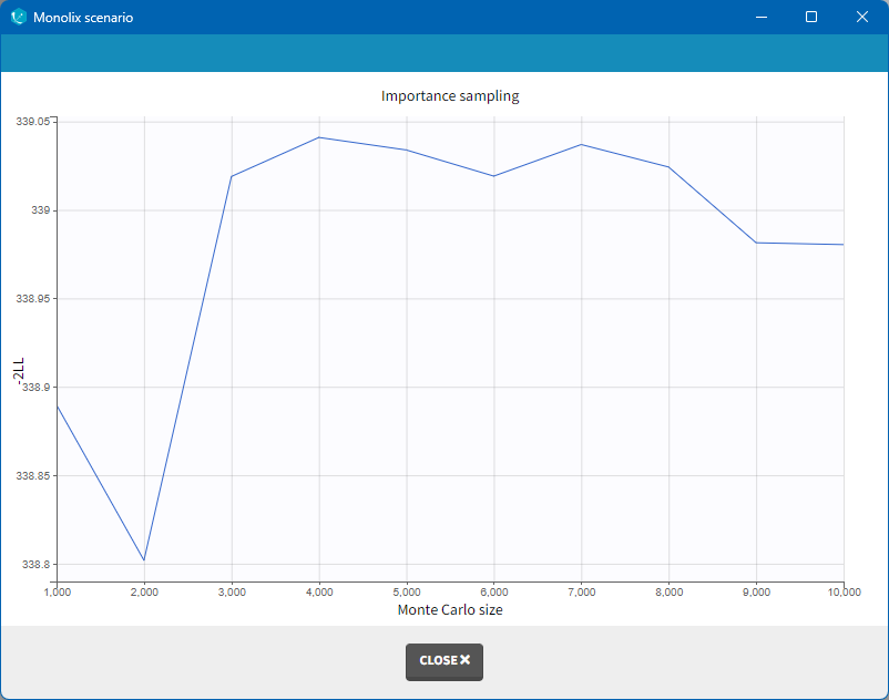
Display and outputs
In case of estimation using the importance sampling method, a graphical representation is proposed to see the valuation of the mean value over the Monte Carlo iterations as on the following:
The final estimations are displayed in the result frame as below. Notice that there is a “Copy table” icon on the top of each table to copy them in Excel, Word, … The table format and display will be kept.
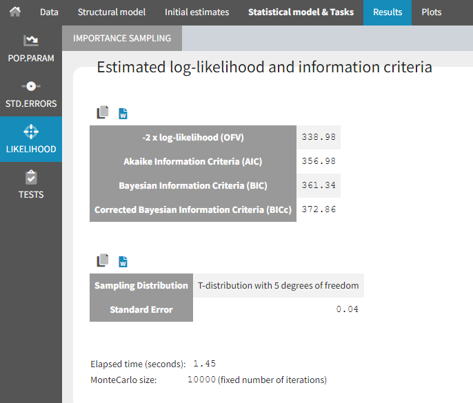
The log-likelihood is given in Monolix together with the Akaike information criterion (AIC) and Bayesian information criterion (BIC):
'%3e%3cg transform='translate(167%2c0)'%3e%3cg transform='translate(-13%2c0)'%3e%3cg transform='translate(9%2c695)'%3e%3cuse xlink:href='%23MJMATHI-41' x='0' y='0'%3e%3c/use%3e%3cuse xlink:href='%23MJMATHI-49' x='750' y='0'%3e%3c/use%3e%3cuse xlink:href='%23MJMATHI-43' x='1255' y='0'%3e%3c/use%3e%3c/g%3e%3cg transform='translate(0%2c-864)'%3e%3cuse xlink:href='%23MJMATHI-42' x='0' y='0'%3e%3c/use%3e%3cuse xlink:href='%23MJMATHI-49' x='759' y='0'%3e%3c/use%3e%3cuse xlink:href='%23MJMATHI-43' x='1264' y='0'%3e%3c/use%3e%3c/g%3e%3c/g%3e%3cg transform='translate(2012%2c0)'%3e%3cg transform='translate(0%2c695)'%3e%3cuse xlink:href='%23MJMAIN-3D' x='277' y='0'%3e%3c/use%3e%3cuse xlink:href='%23MJMAIN-2212' x='1334' y='0'%3e%3c/use%3e%3cuse xlink:href='%23MJMAIN-32' x='2112' y='0'%3e%3c/use%3e%3cg transform='translate(2613%2c0)'%3e%3cuse xlink:href='%23MJCAL-4C' x='0' y='0'%3e%3c/use%3e%3cuse xlink:href='%23MJCAL-4C' x='690' y='0'%3e%3c/use%3e%3cuse transform='scale(0.707)' xlink:href='%23MJMATHI-79' x='1953' y='-213'%3e%3c/use%3e%3c/g%3e%3cuse xlink:href='%23MJMAIN-28' x='4445' y='0'%3e%3c/use%3e%3cg transform='translate(4835%2c0)'%3e%3cuse xlink:href='%23MJMATHI-3B8' x='15' y='0'%3e%3c/use%3e%3cuse xlink:href='%23MJMAIN-5E' x='83' y='268'%3e%3c/use%3e%3c/g%3e%3cuse xlink:href='%23MJMAIN-29' x='5419' y='0'%3e%3c/use%3e%3cuse xlink:href='%23MJMAIN-2B' x='6030' y='0'%3e%3c/use%3e%3cuse xlink:href='%23MJMAIN-32' x='7031' y='0'%3e%3c/use%3e%3cuse xlink:href='%23MJMATHI-50' x='7532' y='0'%3e%3c/use%3e%3c/g%3e%3cg transform='translate(0%2c-864)'%3e%3cuse xlink:href='%23MJMAIN-3D' x='277' y='0'%3e%3c/use%3e%3cuse xlink:href='%23MJMAIN-2212' x='1334' y='0'%3e%3c/use%3e%3cuse xlink:href='%23MJMAIN-32' x='2112' y='0'%3e%3c/use%3e%3cg transform='translate(2613%2c0)'%3e%3cuse xlink:href='%23MJCAL-4C' x='0' y='0'%3e%3c/use%3e%3cuse xlink:href='%23MJCAL-4C' x='690' y='0'%3e%3c/use%3e%3cuse transform='scale(0.707)' xlink:href='%23MJMATHI-79' x='1953' y='-213'%3e%3c/use%3e%3c/g%3e%3cuse xlink:href='%23MJMAIN-28' x='4445' y='0'%3e%3c/use%3e%3cg transform='translate(4835%2c0)'%3e%3cuse xlink:href='%23MJMATHI-3B8' x='15' y='0'%3e%3c/use%3e%3cuse xlink:href='%23MJMAIN-5E' x='83' y='268'%3e%3c/use%3e%3c/g%3e%3cuse xlink:href='%23MJMAIN-29' x='5419' y='0'%3e%3c/use%3e%3cuse xlink:href='%23MJMAIN-2B' x='6030' y='0'%3e%3c/use%3e%3cuse xlink:href='%23MJMATHI-6C' x='7031' y='0'%3e%3c/use%3e%3cuse xlink:href='%23MJMATHI-6F' x='7330' y='0'%3e%3c/use%3e%3cuse xlink:href='%23MJMATHI-67' x='7815' y='0'%3e%3c/use%3e%3cuse xlink:href='%23MJMAIN-28' x='8296' y='0'%3e%3c/use%3e%3cuse xlink:href='%23MJMATHI-4E' x='8685' y='0'%3e%3c/use%3e%3cuse xlink:href='%23MJMAIN-29' x='9574' y='0'%3e%3c/use%3e%3cuse xlink:href='%23MJMATHI-50' x='9963' y='0'%3e%3c/use%3e%3c/g%3e%3c/g%3e%3c/g%3e%3c/g%3e%3c/svg%3e)
where P is the total number of parameters to be estimated and N the number of subjects.
The new BIC criterion penalizes the size of
(which represents random effects and fixed covariate effects involved in a random model for individual parameters) with the log of the number of subjects (
) and the size of
(which represents all other fixed effects, so typical values for parameters in the population, beta parameters involved in a non-random model for individual parameters, as well as error parameters) with the log of the total number of observations (
'%3e%3cg transform='translate(167%2c0)'%3e%3cg transform='translate(-13%2c0)'%3e%3cg transform='translate(0%2c-50)'%3e%3cuse xlink:href='%23MJMATHI-6E' x='0' y='0'%3e%3c/use%3e%3cg transform='translate(600%2c-150)'%3e%3cuse transform='scale(0.707)' xlink:href='%23MJMATHI-74' x='0' y='0'%3e%3c/use%3e%3cuse transform='scale(0.707)' xlink:href='%23MJMATHI-6F' x='361' y='0'%3e%3c/use%3e%3cuse transform='scale(0.707)' xlink:href='%23MJMATHI-74' x='847' y='0'%3e%3c/use%3e%3c/g%3e%3c/g%3e%3c/g%3e%3c/g%3e%3c/g%3e%3c/svg%3e) ), as follows:
), as follows:
'%3e%3cg transform='translate(167%2c0)'%3e%3cg transform='translate(-13%2c0)'%3e%3cg transform='translate(0%2c-84)'%3e%3cuse xlink:href='%23MJMATHI-42' x='0' y='0'%3e%3c/use%3e%3cuse xlink:href='%23MJMATHI-49' x='759' y='0'%3e%3c/use%3e%3cg transform='translate(1264%2c0)'%3e%3cuse xlink:href='%23MJMATHI-43' x='0' y='0'%3e%3c/use%3e%3cuse transform='scale(0.707)' xlink:href='%23MJMATHI-63' x='1011' y='-213'%3e%3c/use%3e%3c/g%3e%3cuse xlink:href='%23MJMAIN-3D' x='2663' y='0'%3e%3c/use%3e%3cuse xlink:href='%23MJMAIN-2212' x='3720' y='0'%3e%3c/use%3e%3cuse xlink:href='%23MJMAIN-32' x='4498' y='0'%3e%3c/use%3e%3cg transform='translate(4999%2c0)'%3e%3cuse xlink:href='%23MJCAL-4C' x='0' y='0'%3e%3c/use%3e%3cuse xlink:href='%23MJCAL-4C' x='690' y='0'%3e%3c/use%3e%3cuse transform='scale(0.707)' xlink:href='%23MJMATHI-79' x='1953' y='-213'%3e%3c/use%3e%3c/g%3e%3cuse xlink:href='%23MJMAIN-28' x='6831' y='0'%3e%3c/use%3e%3cg transform='translate(7221%2c0)'%3e%3cuse xlink:href='%23MJMATHI-3B8' x='15' y='0'%3e%3c/use%3e%3cuse xlink:href='%23MJMAIN-5E' x='83' y='268'%3e%3c/use%3e%3c/g%3e%3cuse xlink:href='%23MJMAIN-29' x='7805' y='0'%3e%3c/use%3e%3cuse xlink:href='%23MJMAIN-2B' x='8416' y='0'%3e%3c/use%3e%3cg transform='translate(9417%2c0)'%3e%3cuse xlink:href='%23MJMAIN-64'%3e%3c/use%3e%3cuse xlink:href='%23MJMAIN-69' x='556' y='0'%3e%3c/use%3e%3cuse xlink:href='%23MJMAIN-6D' x='835' y='0'%3e%3c/use%3e%3c/g%3e%3cuse xlink:href='%23MJMAIN-28' x='11086' y='0'%3e%3c/use%3e%3cg transform='translate(11475%2c0)'%3e%3cuse xlink:href='%23MJMATHI-3B8' x='0' y='0'%3e%3c/use%3e%3cuse transform='scale(0.707)' xlink:href='%23MJMATHI-52' x='663' y='-213'%3e%3c/use%3e%3c/g%3e%3cuse xlink:href='%23MJMAIN-29' x='12582' y='0'%3e%3c/use%3e%3cg transform='translate(13138%2c0)'%3e%3cuse xlink:href='%23MJMAIN-6C'%3e%3c/use%3e%3cuse xlink:href='%23MJMAIN-6F' x='278' y='0'%3e%3c/use%3e%3cuse xlink:href='%23MJMAIN-67' x='779' y='0'%3e%3c/use%3e%3c/g%3e%3cuse xlink:href='%23MJMATHI-4E' x='14584' y='0'%3e%3c/use%3e%3cuse xlink:href='%23MJMAIN-2B' x='15695' y='0'%3e%3c/use%3e%3cg transform='translate(16695%2c0)'%3e%3cuse xlink:href='%23MJMAIN-64'%3e%3c/use%3e%3cuse xlink:href='%23MJMAIN-69' x='556' y='0'%3e%3c/use%3e%3cuse xlink:href='%23MJMAIN-6D' x='835' y='0'%3e%3c/use%3e%3c/g%3e%3cuse xlink:href='%23MJMAIN-28' x='18364' y='0'%3e%3c/use%3e%3cg transform='translate(18753%2c0)'%3e%3cuse xlink:href='%23MJMATHI-3B8' x='0' y='0'%3e%3c/use%3e%3cuse transform='scale(0.707)' xlink:href='%23MJMATHI-46' x='663' y='-213'%3e%3c/use%3e%3c/g%3e%3cuse xlink:href='%23MJMAIN-29' x='19853' y='0'%3e%3c/use%3e%3cg transform='translate(20409%2c0)'%3e%3cuse xlink:href='%23MJMAIN-6C'%3e%3c/use%3e%3cuse xlink:href='%23MJMAIN-6F' x='278' y='0'%3e%3c/use%3e%3cuse xlink:href='%23MJMAIN-67' x='779' y='0'%3e%3c/use%3e%3c/g%3e%3cg transform='translate(21855%2c0)'%3e%3cuse xlink:href='%23MJMATHI-6E' x='0' y='0'%3e%3c/use%3e%3cg transform='translate(600%2c-150)'%3e%3cuse transform='scale(0.707)' xlink:href='%23MJMATHI-74' x='0' y='0'%3e%3c/use%3e%3cuse transform='scale(0.707)' xlink:href='%23MJMATHI-6F' x='361' y='0'%3e%3c/use%3e%3cuse transform='scale(0.707)' xlink:href='%23MJMATHI-74' x='847' y='0'%3e%3c/use%3e%3c/g%3e%3c/g%3e%3c/g%3e%3c/g%3e%3c/g%3e%3c/g%3e%3c/svg%3e)
'%3e%3cg transform='translate(167%2c0)'%3e%3cg transform='translate(-13%2c0)'%3e%3cg transform='translate(0%2c-25)'%3e%3cuse xlink:href='%23MJMATHI-64' x='0' y='0'%3e%3c/use%3e%3cuse xlink:href='%23MJMATHI-69' x='523' y='0'%3e%3c/use%3e%3cuse xlink:href='%23MJMATHI-6D' x='869' y='0'%3e%3c/use%3e%3cuse xlink:href='%23MJMAIN-28' x='1747' y='0'%3e%3c/use%3e%3cg transform='translate(2137%2c0)'%3e%3cuse xlink:href='%23MJMATHI-3B8' x='0' y='0'%3e%3c/use%3e%3cuse transform='scale(0.707)' xlink:href='%23MJMATHI-52' x='663' y='-213'%3e%3c/use%3e%3c/g%3e%3cuse xlink:href='%23MJMAIN-29' x='3243' y='0'%3e%3c/use%3e%3c/g%3e%3c/g%3e%3c/g%3e%3c/g%3e%3c/svg%3e) counts the number of estimated population parameters corresponding to omega_* (standard deviation of IIV), gamma_* (standard deviation of IOV), corr_*_* (correlation between random effects) and beta_* (covariate effects) if the covariate is added on a parameter with random effects.
counts the number of estimated population parameters corresponding to omega_* (standard deviation of IIV), gamma_* (standard deviation of IOV), corr_*_* (correlation between random effects) and beta_* (covariate effects) if the covariate is added on a parameter with random effects.
counts the number of population parameters corresponding to *_pop (typical value), a/b (error model), and betas_* if the covariate is added on a parameter without random effects.
If the log-likelihood has been computed by importance sampling, the number of degrees of freedom used for the proposal t-distribution (5 by default) is also displayed, together with the standard error of the LL on the individual parameters drawn from the t-distribution.
In terms of output, a folder called LogLikelihood is created in the result folder where the following files are created
-
logLikelihood.txt: containing for each computed method, the -2 x log-likelihood, the Akaike Information Criteria (AIC), the Bayesian Information Criteria (BIC), and the corrected Bayesian Information Criteria (BICc).
-
individualLL.txt: containing the -2 x log-likelihood for each individual for each computed method.
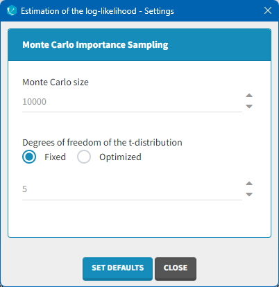
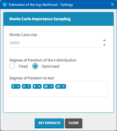
Advanced settings for the log-likelihood
Monolix uses a t-distribution as proposal. By default, the number of degrees of freedom of this distribution is fixed to 5. In the settings of the task, it is also possible to optimize the number of degrees of freedom. In such a case, the default possible values are 1, 2, 5, 10 and 20 degrees of freedom. A distribution with a small number of degree of freedom (i.e. heavy tails) should be avoided in case of stiff ODE’s defined models.