Example

In the proposed example, we use Sycomore to guide the modelling of the PKPD of remifentanil in Monolix, by providing and overview of the modelling workflow, and allowing to easily add a new step of the workflow by cloning a project to modify it.

We choose to perform a quick modelling workflow with the help of automatic model building tools, to find a good model in only a few steps.

All modelling decisions are only summarized.

Insights from data exploration

A detailed presentation and exploration of the remifentanil PKPD dataset that we wish to model is available here.

In summary, it contains:

• administration information for IV infusion,

• PK measurements of remifentanil: these observations are named y1 in Datxplore and Monolix,

• EEG measurements as PD: these observations are named y2 in Datxplore and Monolix,

• continuous covariates (age and lean body mass LBM), as well as categorical covariates (sex and tinfcat which is a dose group).

Data exploration with the data viewer in Monolix gives relevant insights to guide the modelling, mainly:

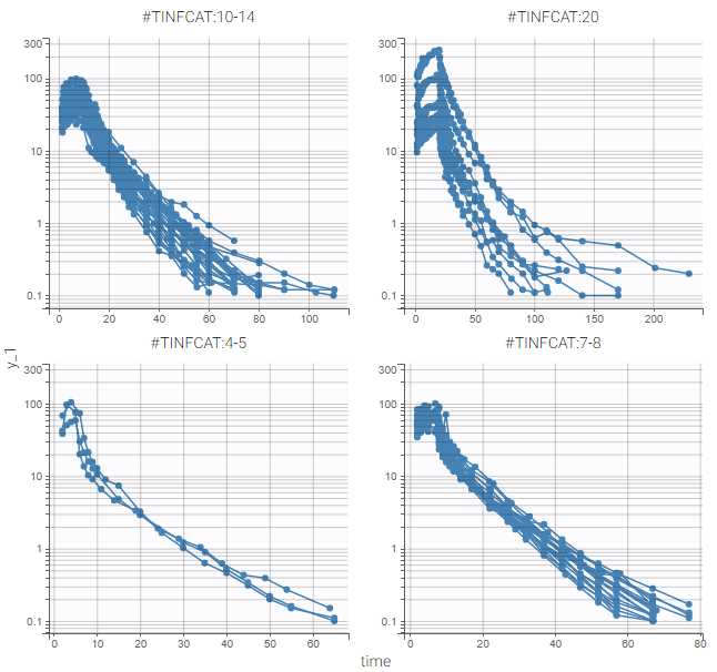
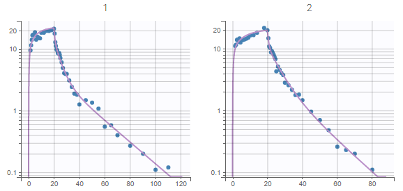
• The elimination shows different phases, as can be seen on the left figure below, where the PK measurements over times have been split by dose group. This means that several compartments will be needed in the PK model to capture them.

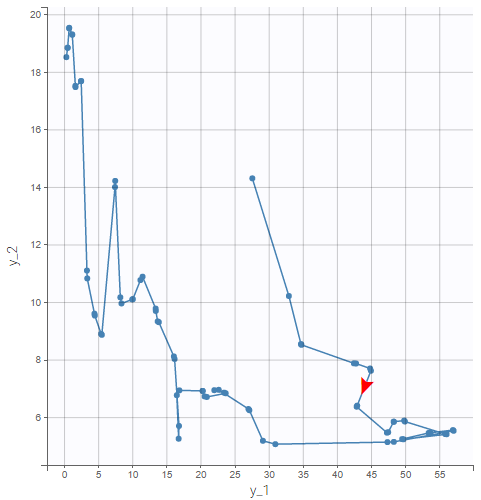
• The PD is inhibited by the PK with a delay, visible for example on the right figure below, which shows the PD over PK for id 15.

First PK model

Since the data exploration in Monolix shows that a model with several compartments seems necessary to describe this dataset, we start by setting up a first PK model with two compartments in Monolix, with the following steps:

• Load the structural model infusion_2cpt_ClV1QV2.txt from the PK library. This is a 2 compartments model with infusion administration and linear elimination.

• Choose automatically good initial estimates for the population parameters with the “Auto-init” button in the tab “Initial estimates”.

• Keep the default statistical model.

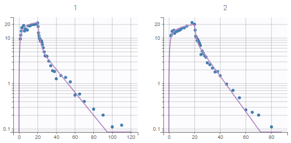
We save this first project as PK_1.mlxtran in a folder “PK”. Then, all estimation and diagnosis tasks are run to evaluate the model. In particular, the plots “Individual fits” and “Observations vs predictions” displayed below show a mis-specification of the structural model: a third compartment is needed in order to avoid under-predictions of the end of the elimination phase.

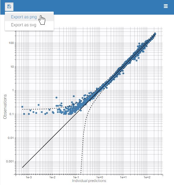
Since these plots are important to diagnose the model, we export these plots in the result folder with the button “Export as png”.

Finally, we note in the tab Comments the conclusion for this project: “Misspecification in diagnostic plots: 3rd cpt needed”.

Second PK model

Next, we change the structural model to add a third compartment to the PK model. This is done by loading the structural model infusion_2cpt_ClV1Q2V2Q3V2.txt. Good initial estimates are again chosen with the button “Auto-init”.

We then save the modified project as PK_2.mlxtran in the PK folder, before running all estimation and diagnosis tasks.

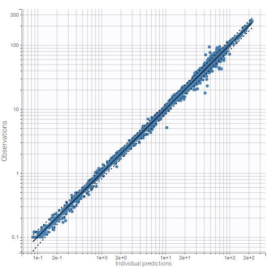
The plots “Individual fits” and “Observations vs predictions” displayed below no longer show any mis-specification of the structural model.

These plots are also exported in the Results folder. Moreover, we note in Comments: “No misspecification in structural model”.

We can also check in the plots for individual parameters that the distributions of the individual parameters are not misspecified.

Comparing two PK projects in Sycomore

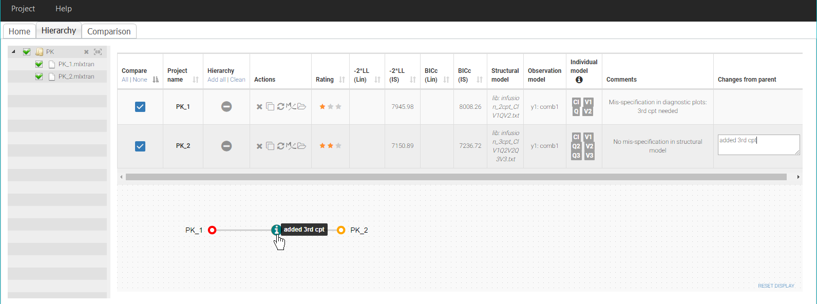
To compare further these two projects, we create a new overview with Sycomore: after opening Sycomore and clicking on “New project”, we select the PK folder containing the two Monolix projects.

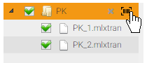
The two projects with their common folder then appear in the Selection panel on the left of the Hierarchy tab in Sycomore. After selecting them both, they also appear with their characteristics in the overview table on the top:

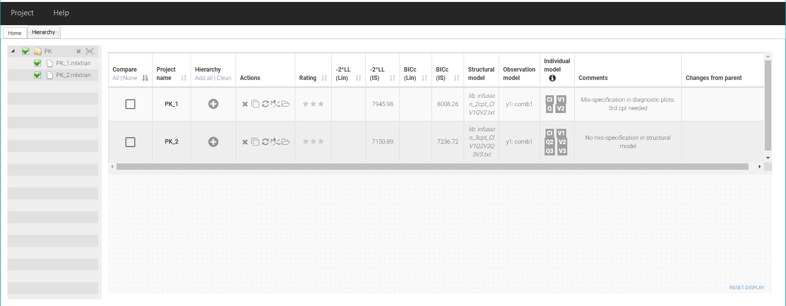
Since both projects contain the BICc computed by importance sampling, we can already see in the table that the second project PK_2 has a lower value for BICc (IS), which confirms that the fit is better. A rating can be added for each project. Here we note a rating ⭐ for PK_1 and a rating ⭐⭐ for PK_2.

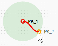
To keep track of the workflow, add these two projects in the tree view by clicking on the + icons in the column “Hierarchy”. The rating appears as a color code, with PK_1 in red and PK_2 in orange. We then drag the node PK_2 close to PK_1 to create a parent-child relationship.

It is now possible to comment the parent-child relationship to record the changes from the parent. We write “added 3rd cpt” in the corresponding cell in the table.

We have now recorded all elements of the current workflow, thus we save the Sycomore overview as a file PKPD_remifentanil.syc. The project now looks like this:

Comparing PK_1 and PK_2 in more details is also possible by selecting them both in the column Compare. The tab Comparison is then generated and allows a side-by-side comparison of the results of the projects.

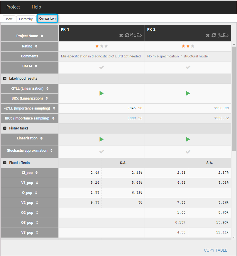
The estimates for Cl, V1 and V2 are quite close between the two projects.

The columns can be sorted according to the values of each row, and missing tasks can also be launched from there with the “run” buttons, for example if the log-likelihood has not been yet computed.

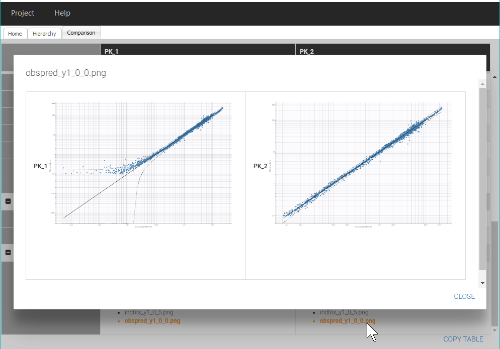
The exported plots in the section Figures can also be compared, for example as below by clicking on obspred_y1_0_0.png, which is the file name for the plot “Observation vs predictions”:

Note that we only mention a few diagnostic plots in this short case study to keep a simple workflow, however it is important to check all diagnostic plots to get a complete model diagnostic.

Adjusting the statistical model with Proposal

The structural model in PK_2 has been validated by the diagnostic plots and parameter estimation. We can now try to improve the statistical model with a different error model, covariate effects or correlations between random effects.

In a complete and detailed modelling workflow, it would be important to look at the diagnostic plots for correlations between covariates and individual parameters as well as between pairs of random effects, to detect possible effects of outliers or to identify relevant transformations for covariates before adding covariate effects. This step is neglected in this simple workflow.

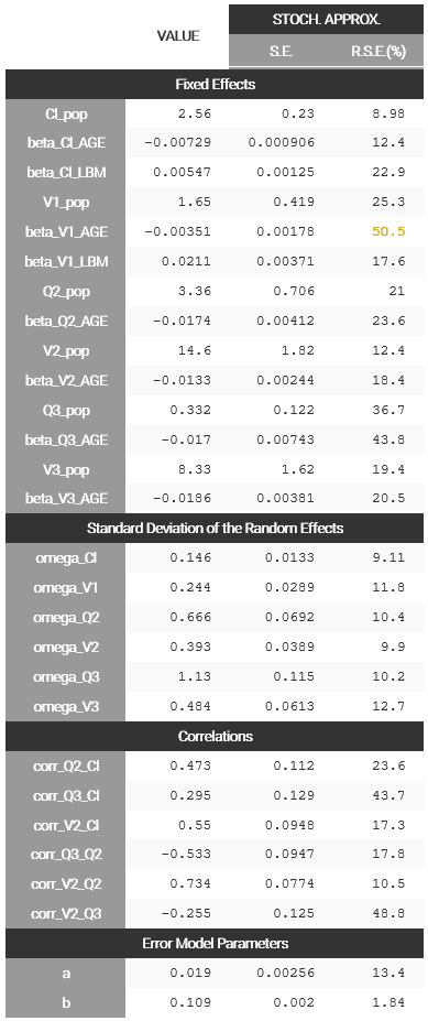
For a quick improvement of the statistical model, we can look at the proposal section in the tab Results of PK_2, seen below. The aim of the Proposal is to estimate the best statistical model for the dataset, taking into account the residual error model, covariate effects and correlations between random effects.

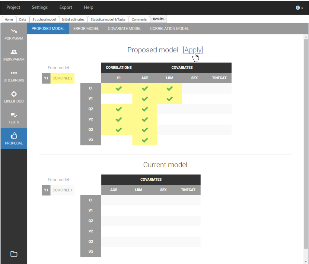
A model different than the current model is available in the tab Proposal. This proposed model includes a combined2 residual error model, covariate effects of Age on all parameters and LBM on Cl and V1, and a correlation group with the random effects of Cl, Q2, V2 and Q3. It is estimated that this model will be more performant than the current model, thus it is an interesting information that we can add in the Comments for PK_2.mlxtran with: “Statistical model can be improved”. We save PK_2.mlxtran to update its comments, and we can also update the Comments visible in Sycomore by clicking on the “refresh” button for PK_2 in the column Actions:

However the performance of the proposed model should be verified by applying the model and estimating its parameters.

To do this, we choose the proposed model in Monolix by clicking on “Apply”, and save the modified project as PK_3.mlxtran. We run the scenario of tasks for this project, and check that the convergence of the estimates is good and that all parameters are estimated with a good confidence:

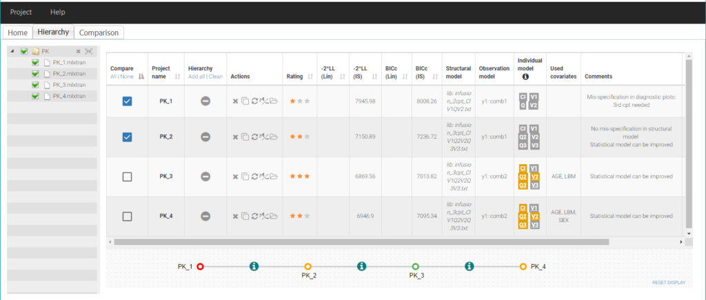
Next, we add PK_3 in the workflow overview to compare it to the previous projects, by clicking on the icon “Rescan directory” next to the PK folder in the Selection panel, like this:

This adds the project PK_3.mlxtran in the list of selected projects of the overview. It can now be added in the tree view as a child of PK_2, with the comment “Applied best proposal”.

As we can see on the table below, the BICc indeed indicates that PK_3 is more performant than PK_2, thus we choose the rating ⭐⭐⭐ for PK_3. Note that BICc values can be easily compared in this table by sorting the column BICc with the button marked on the figure.

In the tab Results of Monolix for PK_3, we see that PK_3 also has a proposed model available, where a covariate effect of Sex is also included on V3, therefore, we finalize PK_3 with a comment “Proposed model available” and save.

If the proposal at the previous step has been efficient, we should not expect a large improvement of the objective function value with this new covariate effect. To check this, we apply again the best proposed model and save the modifications in a project PK_4.mlxtran. As before, it is important to not only run the scenario, but also check the convergence of the estimates and their standard errors.

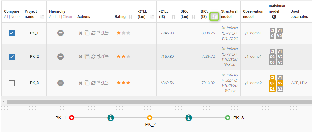
Once this is done, we add PK_4 to the overview in Sycomore. Since the table is still sorted by BICc, it is quickly visible that PK_4 actually has a higher BICc than PK_3. Therefore, we choose a rating ⭐⭐ for PK_4 and we consider PK_3 as more performant.

We can now consider PK_3 as the final PK model. To save this decision in the comments of the project, it is possible to open again the project in Monolix directly from Sycomore, by clicking on the “Monolix” icon in the row for PK_3:

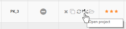
After completing the comments and saving the project, the comments displayed in Sycomore can be updated with the “refresh” button.

Joint PK-PD model

We next would like to develop a joint model for the PK and the PD. We choose to try two different PD models that could take into account the delay between remifentanil concentration and decrease of EEG, revealed by the data exporation:

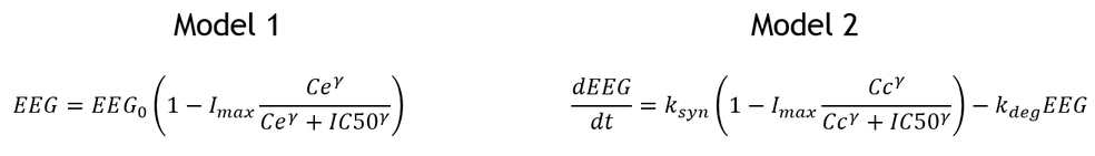
• Model 1: a direct inhibition model with an effect compartment.

• Model 2: a turnover model with PD production inhibition by the PK.

Here are the equations for EEG (PD observations) for both models:

We will now define two projects with these two models, available in the libraries of Monolix, and we will then run the two projects in a row from Sycomore.

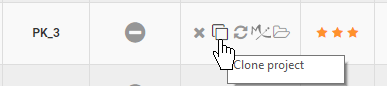
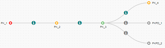
Since both PKPD models will be based on the final PK model, we start by creating two clones of PK_3 in Sycomore with the button “Clone project” (note that the action “Clone project” is also available by clicking on the node for PK_3 in the tree view):

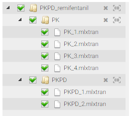
We save each cloned project in a new folder named PKPD, under the names PKPD_1.mlxtran and PKPD_2.mlxtran. The cloned project are automatically included in the panel selection and the tree view as children nodes of PK_3:

Let’s now open PKPD_1.mlxtran in Monolix to add the first PD model.

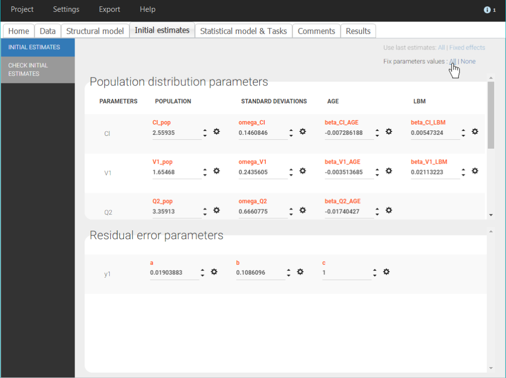
The project has been saved with the comments of PK_3, that we can delete, and the results of PK_3, which means that the PK parameters estimated with PK_3 are available. We start by defining these estimated parameters as new initial values, by clicking on “Use last estimates: all”  in the tab “Initial estimates”. Then, we choose to fix all the PK population parameters: the goal is to perform a quick estimation of only the PD population parameters that will be added later in the model. To fix all population parameters, we click on “Fix parameters values: All” in the tab “Initial estimates”:

Note that this method is easy to implement in the interface of Monolix and allows to estimate only the PD population parameters, however all individual parameters will be estimated, including the PK parameters. Therefore, it will take longer than a fully sequential approach where individual PK parameters from the PK analysis are included in the dataset to be used for predictions.

We can now complete the structural model with a PD model. In the tab “Structural model”, we load a model from the PKPD models library, corresponding to the same PK model as before, with a partial inhibition PD model with effect compartment and with sigmoidicity.

We choose good initial values for the PD parameters in the panel “Check initial estimates” of the tab “Initial estimates”. The auto-init is only available for models from the PK library, therefore we have to choose manually some values that give a reasonnable fit to the data, for example ke0_pop=1, gamma_pop=2, E0_pop=20, Imax_pop=0.9, IC50_pop=10. We can then save the modified project. Since the project will be run from Sycomore, we make sure that all the tasks of the scenario are selected and saved.

We follow the same steps as for PKPD_1.mlxtran to define the second PD model in PKPD_2.mlxtran. Here we choose a PKPD model where the PD model is a turnover model with partial inhibition of the production and with sigmoidicity. We can take for initial values kout_pop=1, gamma_pop=2, R0_pop=20, Imax_pop=0.9, IC50_pop=10.

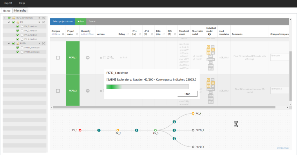
Once both projects have been defined and refreshed in Sycomore, we can launch their scenarios directly from Sycomore, by clicking in the table on the two names PKPD_1 and PKPD_2. The projects are then colored in green. The list of selected projects can then be run in a row with the button “Run”. A pop-up window opens to display the progess of the runs:

After the two runs have finished, we finally select the two PKPD projects for side-by side comparison, to check their results, in particular the estimated values and standard errors. In both cases, the parameters have been estimated with a good confidence.

To compare the diagnostic plots, it is necessary to open the projects in the interface of Monolix to generate the plots and export them as png images. The comparison of the VPC for example shows that both models have a good predictive power:

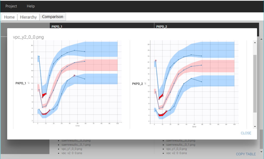
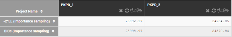
Finally, the comparison of the BICc values indicate that the model 1 is slightly more performant than model 2.

To visualize this difference on the tree view, we choose a rating ⭐⭐⭐ for PKPD_1 and ⭐⭐ for PKPD_2.

Conclusion

We built a quick joint PKPD model for remifentanil in Monolix, with the help of structural model libraries and automatic statistical model building tools implemented in Monolix.

This example illustrates how Sycomore can be used to:

• track the steps of the modelling workflow and see at a glance the main elements of each step,

• easily add a new step of the workflow by cloning a Monolix project,

• save the changes between successive runs,

• compare side-by-side the results of similar models,

• run sets of Monolix projects.

All the material of this case study (data, Monolix projects and Sycomore overview) can be downloaded here: PKPD_remifentanil_workflow_sycomore.zip