Delayed differential equations

Objectives: learn how to implement a model with ordinary differential equations (ODE) and delayed differential equations (DDE).

Demos: tgi_project, seir_project

https://www.youtube.com/watch?v=oliKcm849Wc

Ordinary differential equations based model

tgi_project (data = tgi_data.txt , model = tgi_model.txt)

Here, we consider the tumor growth inhibition (TGI) model proposed by Ribba et al. (Ribba, B., Kaloshi, G., Peyre, M., Ricard, D., Calvez, V., Tod, M., . & Ducray, F., *A tumor growth inhibition model for low-grade glioma treated with chemotherapy or radiotherapy*. Clinical Cancer Research, 18(18), 5071-5080, 2012.). This model is defined by a set of ordinary differential equations

where is the total tumor size. This set of ODEs is valid for t greater than 0, while

This model (derivatives and initial conditions) can easily be implemented with Mlxtran:

CODE

DESCRIPTION: Tumor Growth Inhibition (TGI) model proposed by Ribba et al
A tumor growth inhibition model for low-grade glioma treated with chemotherapy or radiotherapy. 
Clinical Cancer Research, 18(18), 5071-5080, 2012.

Variables 
- PT: proliferative equiescent tissue
- QT: nonproliferative equiescent tissue
- QP: damaged quiescent cells 
- C:  concentration of a virtual drug encompassing the 3 chemotherapeutic components of the PCV regimen

Parameters
- K      : maximal tumor size (should be fixed a priori)
- KDE    : the rate constant for the decay of the PCV concentration in plasma
- kPQ    : the rate constant for transition from proliferation to quiescence
- kQpP   : the rate constant for transfer from damaged quiescent tissue to proliferative tissue 
- lambdaP: the rate constant of growth for the proliferative tissue
- gamma  : the rate of damages in proliferative and quiescent tissue
- deltaQP: the rate constant for elimination of the damaged quiescent tissue
- PT0    : initial proliferative equiescent tissue
- QT0    : initial nonproliferative equiescent tissue

[LONGITUDINAL]
input = {K, KDE, kPQ, kQpP, lambdaP, gamma, deltaQP, PT0, QT0}

PK:
depot(target=C)

EQUATION:
; Initial conditions
t0    = 0
C_0   = 0
PT_0  = PT0
QT_0  = QT0
QP_0  = 0

; Dynamical model
PSTAR   = PT + QT + QP
ddt_C   = -KDE*C
ddt_PT  = lambdaP*PT*(1-PSTAR/K) + kQpP*QP - kPQ*PT - gamma*KDE*PT*C
ddt_QT  = kPQ*PT - gamma*KDE*QT*C
ddt_QP  = gamma*KDE*QT*C - kQpP*QP - deltaQP*QP

OUTPUT:
output = PSTAR

t0, PT_0 and QT_0 are reserved keywords that define the initial conditions.

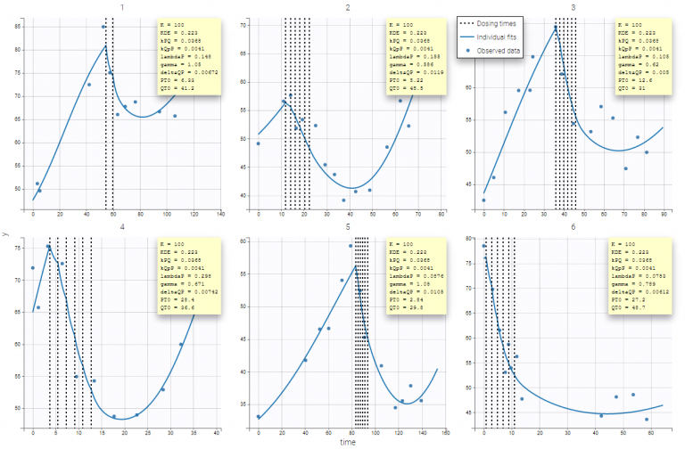
Then, the graphic of individual fits clearly shows that the tumor size is constant until t=0 and starts changing according to the model at t=0.

Don’t forget the initial conditions!

tgiNoT0_project (data = tgi_data.txt , model = tgiNoT0_model.txt)

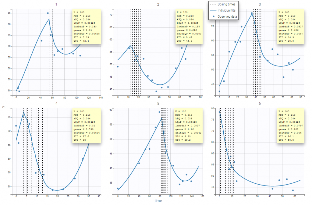
The initial time t0 is not specified in this example. Since t0 is missing, Monolix uses the first time value encountered for each individual. If, for instance, the tumor size has not been computed before 5 for the individual fits, then t0=5 will be used for defining the initial conditions for this individual, which introduces a shift in the plot:

As defined here, the following rule applies

When no starting time t0 is defined in the Mlxtran model for Monolix then by default t0 is selected to be equal to the first dose or the first observation, whatever comes first.
If t0 is defined, a differential equation needs to be defined.

Conclusion: don’t forget to properly specify the initial conditions of a system of ODEs!

Delayed differential equations based model

A system of delay differential equations (DDEs) can be implemented in a block EQUATION of the section [LONGITUDINAL] of a script Mlxtran. Mlxtran provides the command delay(x,T) where x is a one-dimensional component and T is the explicit delay. Therefore, DDEs with a nonconstant past of the form

can be solved. The syntax and rules are explained here.

seir_project (data = seir_data.txt , model = seir_model.txt)

The model is a system of 4 DDEs and defined with the following mode:

CODE

DESCRIPTION: SEIR model, using delayed differential equations.
"An Epidemic Model with Recruitment-Death Demographics and Discrete Delays"�, Genik & van den Driessche (1999)

Decomposition of the total  population into four epidemiological classes 
S (succeptibles), E (exposed), I (infectious), and  R (recovered)

The parameters corresponds to 
- birthRate: the birth rate,
- deathRate: the natural death rate,
- infectionRate: the contact rate of infective individuals,
- recoveryRate: the rate of recovery,
- excessDeathRate: the excess death rate for infective individuals

There is a time delay in the model:
- tauImmunity: a temporary immunity delay

[LONGITUDINAL]
input = {birthRate, deathRate, infectionRate, recoveryRate, excessDeathRate, tauImmunity, tauLatency}

EQUATION:
; Initial conditions
t0    = 0
S_0 = 15
E_0 = 0
I_0  = 2
R_0 = 3

; Dynamical model
N = S + E + I + R

ddt_S = birthRate - deathRate*S - infectionRate*S*I/N + recoveryRate*delay(I,tauImmunity)*exp(-deathRate*tauImmunity)
ddt_E = infectionRate*S*I/N - deathRate*E - infectionRate*delay(S,tauLatency)*delay(I,tauLatency)*exp(-deathRate*tauLatency)/(delay(I,tauLatency)+delay(S,tauLatency)+delay(E,tauLatency)+delay(R,tauLatency))
ddt_I = -(recoveryRate+excessDeathRate+deathRate)*I + infectionRate*delay(S,tauLatency)*delay(I,tauLatency)*exp(-deathRate*tauLatency)/(delay(I,tauLatency)+delay(S,tauLatency)+delay(E,tauLatency)+delay(R,tauLatency))
ddt_R = recoveryRate*I - deathRate*R - recoveryRate*delay(I,tauImmunity)*exp(-deathRate*tauImmunity)

OUTPUT:
output = {S, E, I, R}

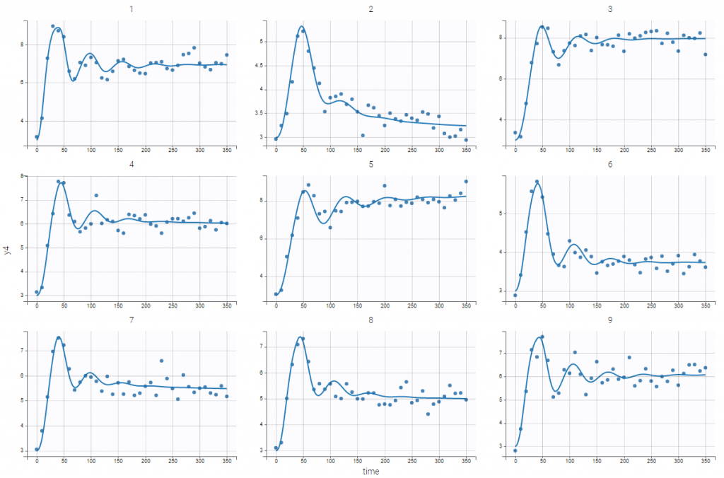
Introducing these delays allows to obtain nice fits for the 4 outcomes, including (corresponding to the output y4):

Case studies

8.case_studies/arthritis_project