Count data models

Related resources on modeling count data in Monolix:

Columns used to define observations: formatting of count data in the MonolixSuite
Count observation model: details on the different models for count data that can be used in Monolix and their syntax
Count data model library: detailed description of the library of count models integrated within Monolix

On the current page, we show examples of count data models from the Monolix demos.

Demos: count1a_project, count1b_project, count2_project

Count data with constant distribution over time

count1a_project (data = ‘count1_data.txt’, model = ‘count_library/poisson_mlxt.txt’)

A Poisson model is used for fitting the data:

CODE

[LONGITUDINAL]
input = lambda

DEFINITION:
Y = {type = count,  log(P(Y=k)) = -lambda + k*log(lambda) - factln(k) }

OUTPUT:
output = Y

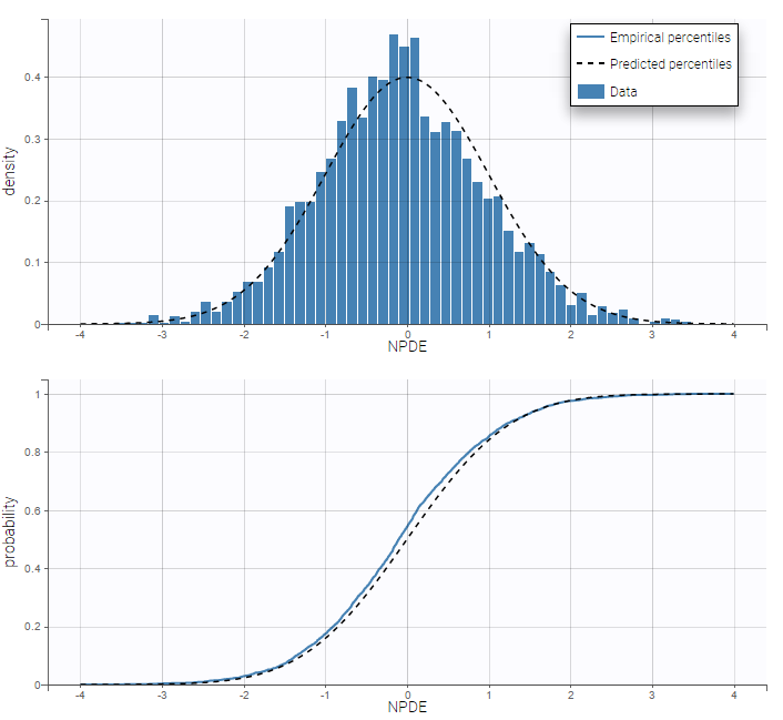
Residuals for noncontinuous data reduce to NPDEs. We can compare the empirical distribution of the NPDEs with the distribution of a standardized normal distribution either with the pdf (top) or the cdf (bottom):

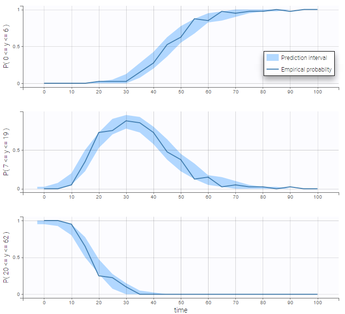
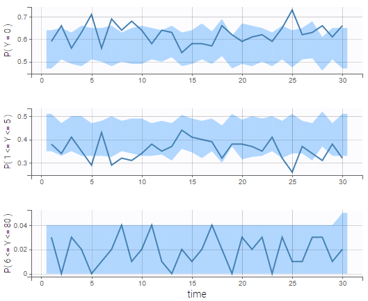
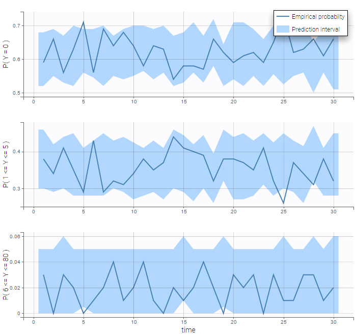
VPCs for count data compare the observed and predicted frequencies of the categorized data over time:

count1b_project (data = ‘count1_data.txt’, model = ‘count_library/poissonMixture_mlxt.txt’)

A mixture of two Poisson distributions is used to fit the same data. For that, we define the probability of k occurrences as the weigthed sum of two Poisson distributions with two expected numbers of occurrences lambda1 and lambda2. The structural model file writes

CODE

[LONGITUDINAL]
input = {lambda1, alpha, mp}

EQUATION:
lambda2 = (1+alpha)*lambda1

DEFINITION:
Y = { type = count,
       P(Y=k) = mp*exp(-lambda1 + k*log(lambda1) - factln(k)) + (1-mp)*exp(-lambda2 + k*log(lambda2) - factln(k)) 
}

OUTPUT:
output = Y

Thus, the parameter alpha has to be strictly positive to ensure different expected number of occurrences in the two poisson distributions and mp has to be in [0, 1] to ensure the probability is correctly defined. Thus those parameters should be defined with lognormal and probitnormal distribution respectively as shown on the following figure.

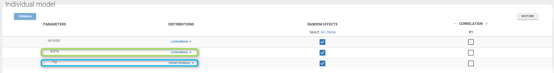
We see on the VPC below that the data set is well modeled using this mixture of Poisson distributions.

Count data with time varying distribution

count2_project (data = ‘count2_data.txt’, model = ‘count_library/poissonTimeVarying_mlxt.txt’)

The distribution of the data changes with time in this example:

We then use a Poisson distribution with a time varying intensity:

CODE

[LONGITUDINAL]
input =  {a,b}
                           
EQUATION:
lambda= a*exp(-b*t)
                           
DEFINITION:
y = {type=count, P(y=k)=exp(-lambda)*(lambda^k)/factorial(k)}

OUTPUT:
output = y

This model seems to fit the data very well: