Library of PK models

The PK library is a library of standard PK models. Instead of writing the structural model yourself, you can select among simple PK models already written for you. When you select the PK library, a full list of all available models appear, which you can filter by selecting options for administration, distribution and elimination.

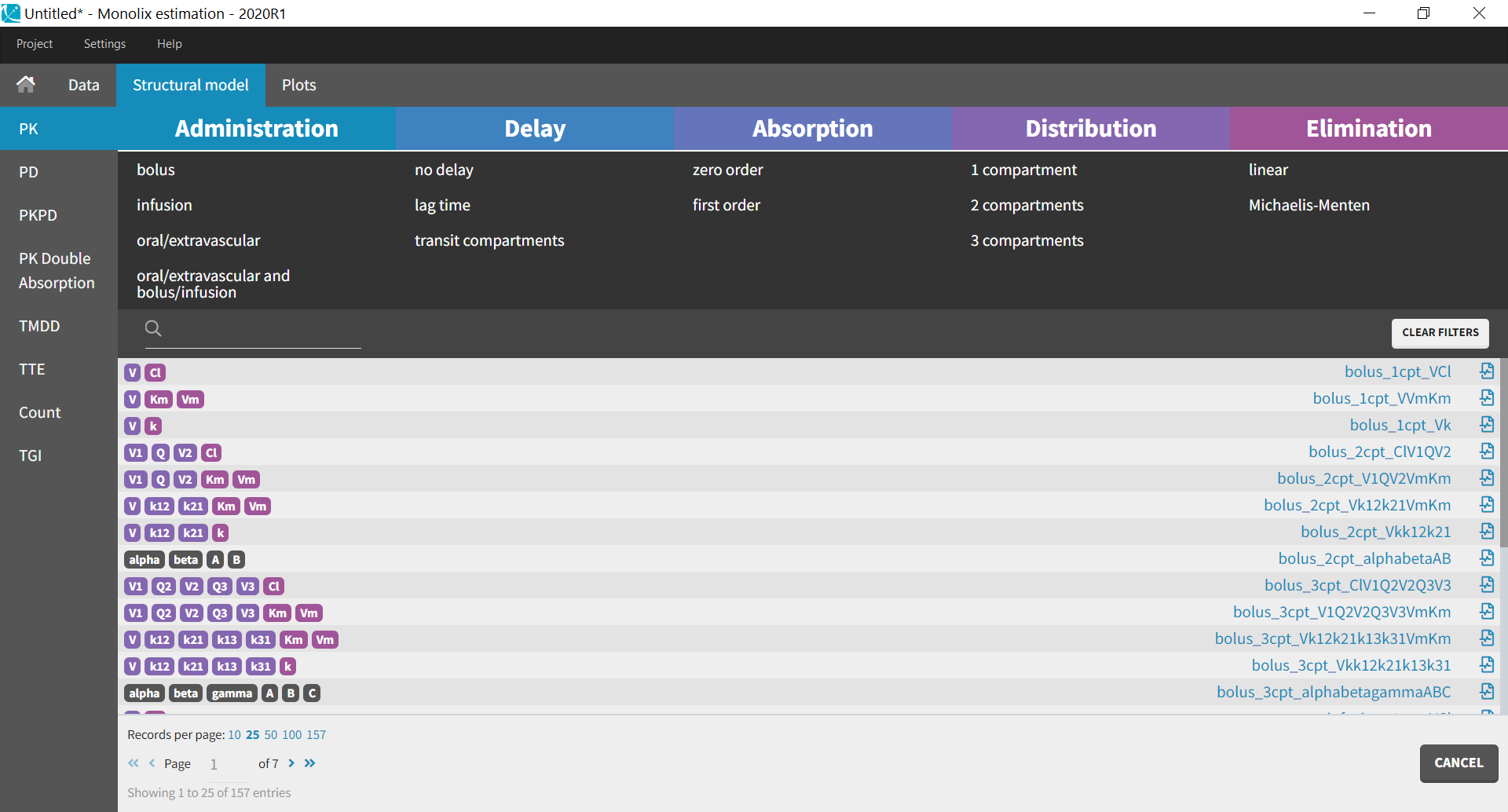
Here we provide general guidelines to guide you towards the standard PK model that is the most suited to your dataset.

If you open any of the .txt files in this library, corresponding to the model written in mlxtran-formatted code, you see that the pkmodel macro is always used. This macro enables to define all standard PK models in a compact manner (except for multiple administration routes). It uses the analytical solution of the ODE system to simulate it, if it is available (which is the case for all models with linear elimination and without transit compartments), and otherwise the ODE system itself. A complete list of the analytical solutions for standard PK and PKPD models is available in this document: PKPDlibrary.pdf

If none of the standard PK models seems to fit your needs, consider using a model from our other PK libraries (PK double absorption, TMDD). To define your own custom PK model, jump directly to data and models.

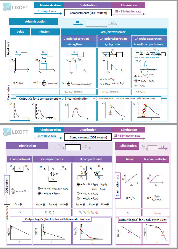
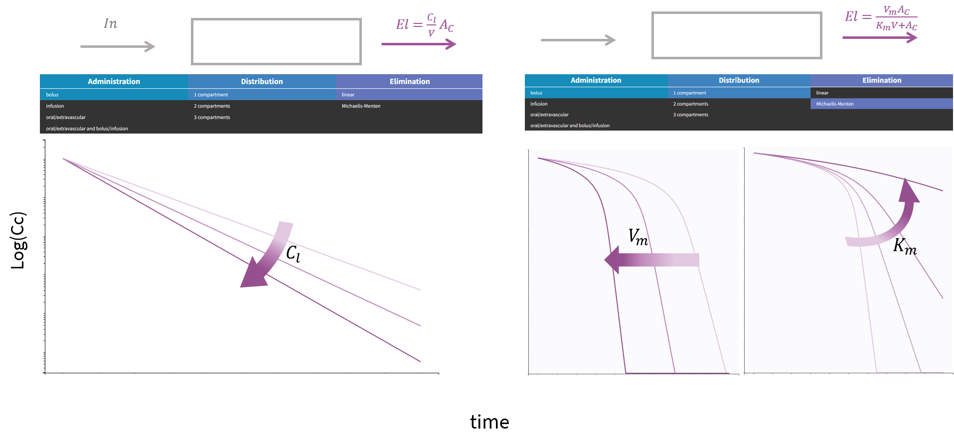
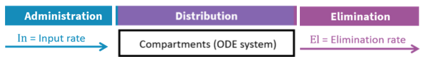
All PK models in the library correspond to a system of equations with the following structure:

• an input rate which depends on the type of administration

• an ODE system based on a number of compartments

• an elimination rate which depends on the type of elimination selected.

The equations express the concentration Cc(t) in the central compartment at a time t after the last drug administration:

• Single dose: at time t after dose D given at time

• Multiples doses: at time t after n doses for i from 1 to n given at time

• Steady state: at a time t after dose D given at time after repeated administration of dose D given at interval (only for linear elimination)

Routes of administration

You should know the type of administration to use based on the study that generated the dataset. The route of administration will determine the dynamics of the input rate In(t) for the system described in Distribution.

To explore the differences in administration routes, we will see how they impact the input rate of a model with 1 compartment and linear elimination, parameterized with the clearance.

The ODE system for this model is:

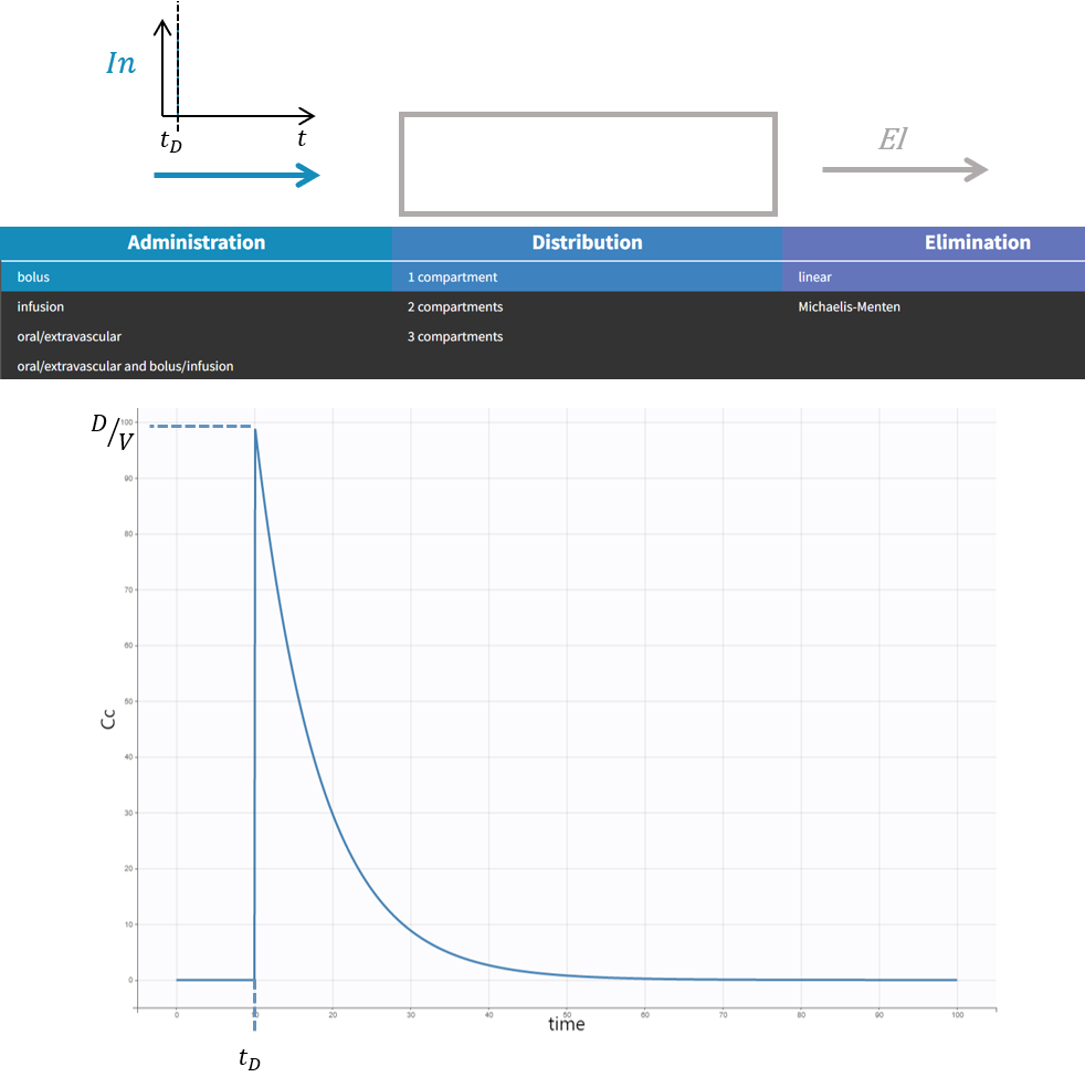
Intravenous bolus

The intravenous bolus is an injection which quickly raises the concentration of the substance in the blood to an effective level. When bolus is selected, if D is the dose administered at time , we set the amount in the central compartment to . This is equivalent to modeling the input rate as a dirac .

The response in the central compartment to a bolus in case of a model with 1 compartment with linear elimination is a decreasing exponential:

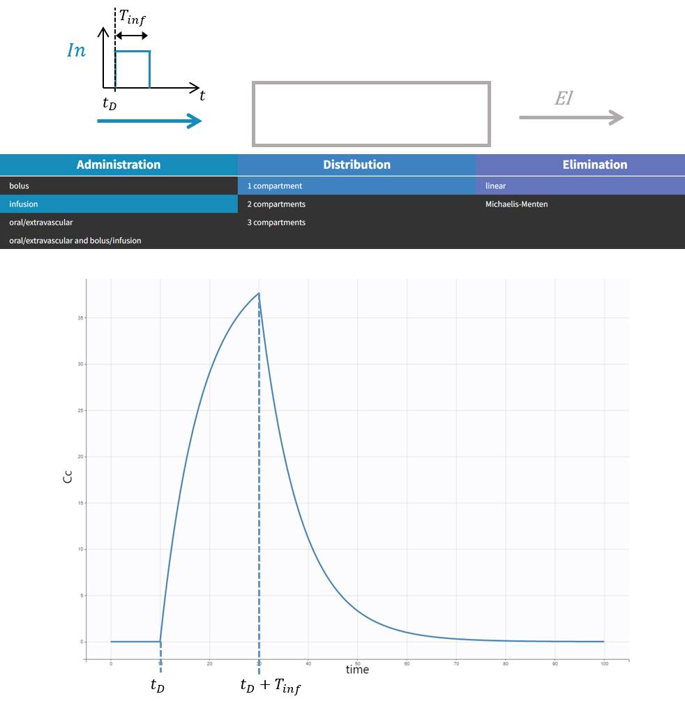
Infusion

This section focuses on intravenous infusion. For subcutaneous infusions, check the dedicated subsection in the oral/extravascular section.

To have the input modeled as an infusion instead of a bolus, you need to have a column tagged as ‘infusion rate’ or ‘infusion duration’ in your dataset in Monolix (the duration will be deduced from the amount and rate columns if rate is specified, and vice versa). In Simulx, you need to create a treatment element that is an infusion.

The intravenous infusion of duration sets the input rate to a constant value during the infusion, and then to zero: .

The response in the central compartment in case of a model with 1 compartment with linear elimination is increasing as soon as the infusion starts, and decreasing as soon as it stops.

Note that bolus and infusion models are encoded exactly the same way with the pkmodel macro. It is the pkmodel macro that will check if a column tagged as INFUSION RATE or INFUSION DURATION appears in the dataset, and if this is the case, use the analytical solution of the infusion equations instead of the bolus equations. 

Oral/extravascular administration

In the case of an oral or extravascular administration, you have additional options for delay and for the type of absorption.

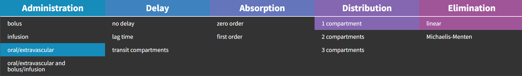
Absorption: 0 or 1st order?

The type of absorption will determine if the peak in the response is sharp or smooth.

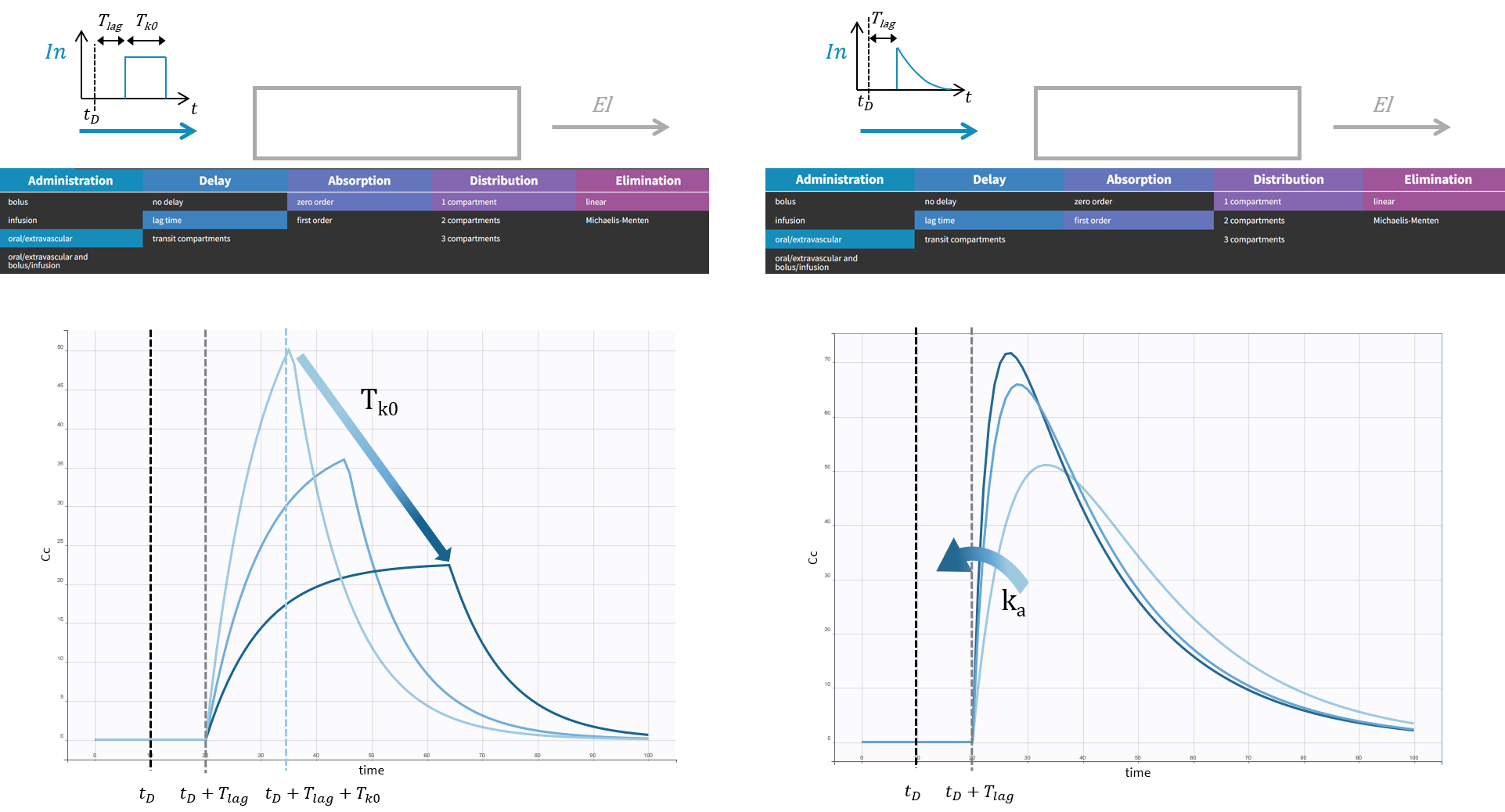
A zero-order absorption is modeled with the same input rate as for an infusion, i.e. with a square pulse input, with 2 differences:

• the duration of the input Tk0 is not known, it is thus part of the parameters to optimize, and it will influence the height and the duration of the response,

• a delay can be added between the dosing time and the start of the pulse, and this delay can also be optimized.

A first-order absorption will instead correspond to a sharper input pulse with a slow exponential decay which depends on the absorption rate. Because of this, the response peak is smoother. This input rate is the analytical solution of a system with a depot compartment where the dose would be added at time , and which would be transferred to the central compartment with an absorption rate ka:

We compare here zero and 1st order absorption in the case of a lag time, but if there is no lag in the response, the no delay option can be selected and the parameter Tlag will disappear.

Delay: lag time or transit compartments?

In the case of a 1st order absorption, it is possible to select between two types of delay: a lag time or transit compartments. The type of delay selected will change the rising phase of the pulse input. A lag time corresponds to an instantaneous increase of the input rate at time whereas transit compartments will lead to a more gradual increase of the input rate right after . The rational for transit compartments and alternative phenomenological models for delayed absorption are described in a specific page. Transit compartments are sometimes more accurate than a lag time but the models take longer to simulate because there is no analytical solution available.

Instead of adding the dose to a depot compartment which would be also the absorption compartment at , the dose is added at but a number of transit compartments with transit rate ktr between the compartments are added between the depot and the absorption compartment.

The input rate is the solution of the following system:

This absorption model gives more flexibility to fit the absorption phase with the 3 following parameters: transit rate ktr, the absorption rate ka and the mean transit time .

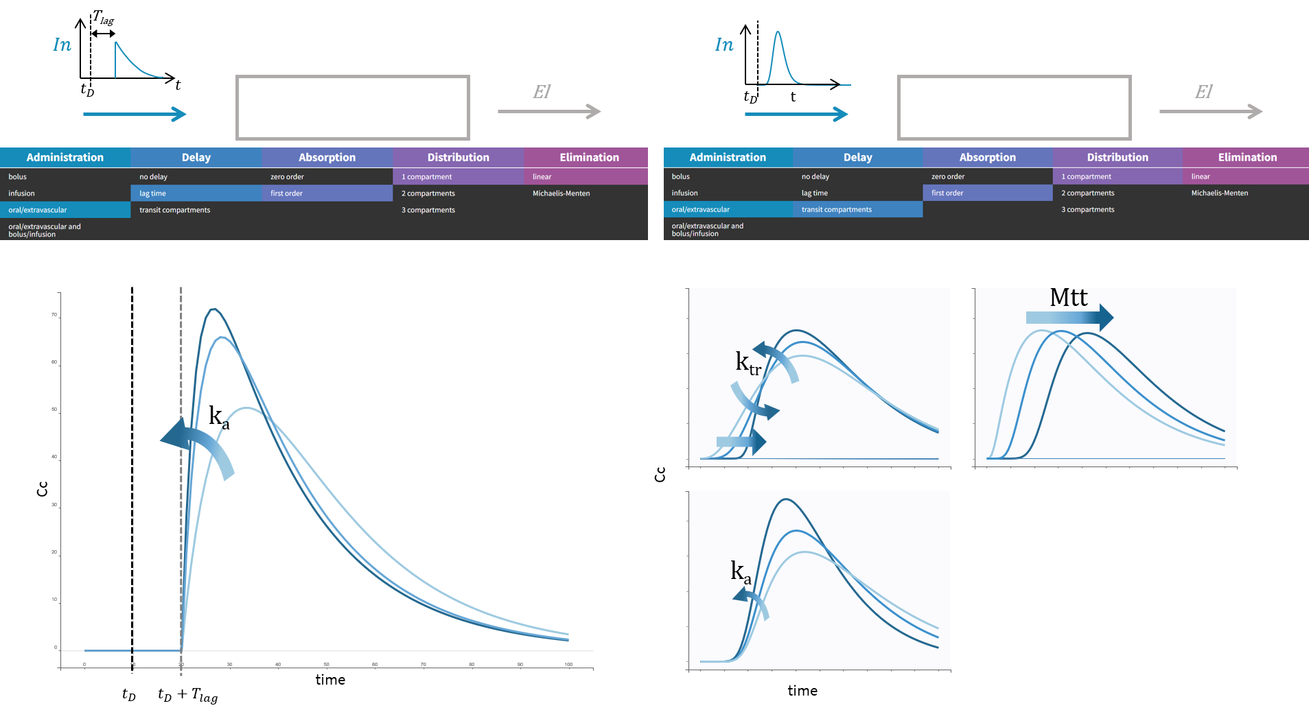
Subcutaneous infusion

To have the input modeled as a subcutaneous infusion, you need to

• select a model with an oral/extravascular administration

• have a column tagged as ‘infusion rate’ or ‘infusion duration’ in your dataset in Monolix (the duration will be deduced from the amount and rate columns if rate is specified, and vice versa), or create a treatment element that is an infusion in Simulx.

Only 1st-order absorption is available in this case, and the input rate in case of Tlag (or no delay, i.e. Tlag = 0) is the solution of the following subsystem, combining the equations described above for infusion and for first-order absorption:

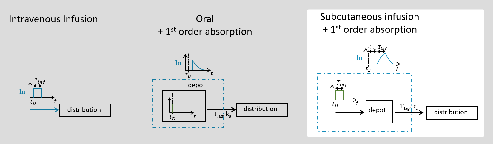
Multiple administration routes

It is possible to use a combination of an oral or extravascular administration, and a bolus or an infusion. For this, a column should be tagged as administration ID in the dataset with 1 for all doses administered  intravenously and  2  for orally or extravascularly administered doses. In this case, the input rate is the sum of:

• an infusion rate if columns tagged as INFUSION RATE or INFUSION DURATION appear in the data, or a bolus rate otherwise,

• a rate for oral administration defined above.

In practice, most of the time the two administrations are not simultaneous and the rate takes in turn the value of a rate for an infusion/bolus and for an oral administration, according to the dosing times in the data set.

For each of the combined models, there is a possibility to incorporate the bioavailability by selecting the model with parameter F. This will multiply the oral/extravascular administration input rate by the number F. We give this possibility only in case of multiple administration routes because in a single route setting, F and V would only appear in the ratio V/F which makes them non-identifiable.

Distribution

The input rate defined by the administration route impacts the amount of drug in the central compartment. You can select to have additional peripheral compartments leading to a system with 1, 2 or 3 compartments in total:

The ODE system for standard PK models involves one species per compartment. The amount of drug in the central compartment is called A_c, and for the 2nd and 3rd compartment it is called A₂ and A_3. The output of the model is the concentration in the central compartment C_c.

The ODE system for each case is given here, parameterized by the volumes in each compartment V1, V2, V3 and the intercompartmental clearance Q.

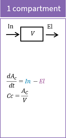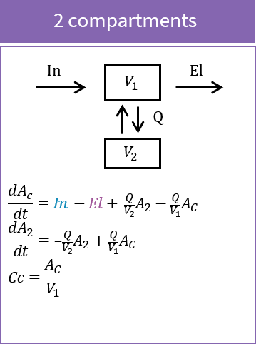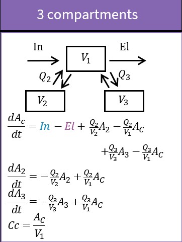Instead of using the intercompartmental clearance Q_i between the central compartment and a peripheral compartment i, and a volume V_i for each compartment, it is also possible to use the volume V in the central compartment only and transfer rates for each peripheral compartmental compartment i: .

In and El rates are defined by the selected administration route and the elimination rate.

To show the impact of the number of compartments, we will see how they impact the response of a model with a bolus and linear elimination, parameterized with the clearance.

Impact of parameters in the case of 1 compartment

In the case of 1 compartment, the ODE system for a bolus with linear elimination parameterized with the clearance for is:

The response is given by a decreasing exponential . If the elimination rate Cl/V is kept constant (to focus on the effect of the distribution parameters), increasing the volume V will translate the whole response down:

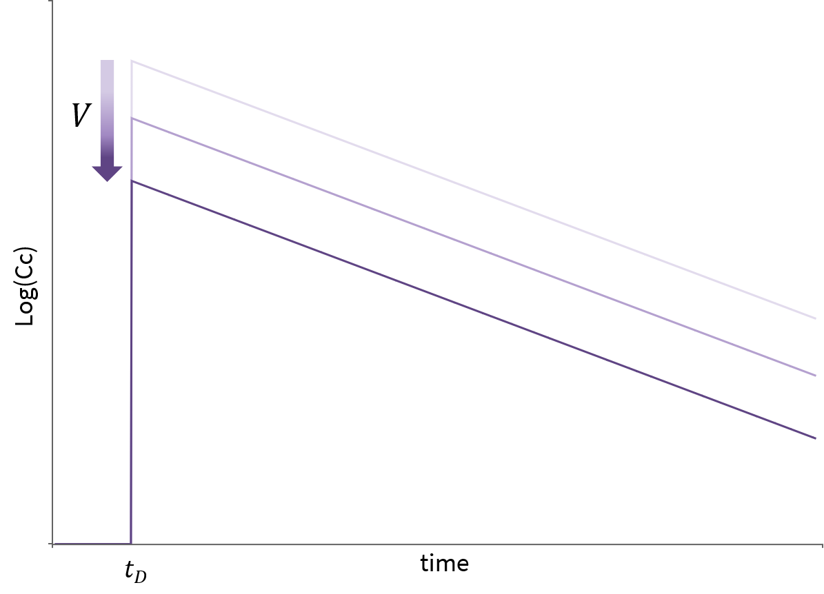
Impact of parameters in the case of 2 compartments

In the case of 2 compartments, the ODE system for a bolus with linear elimination leads to a response involving a sum of decreasing exponentials such that log(Cc shows 2 different slopes. Increasing V1 makes the response start lower, increasing V2 decreases the value at which the slope changes, and increasing Q moves this point earlier, making the slope change also sharper.

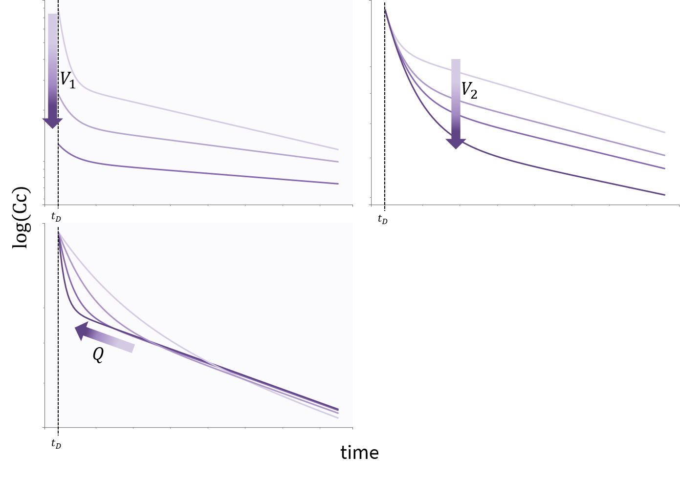
Impact of parameters in the case of 3 compartments

The case of 3 compartments is similar to the case of 2 compartments. log(Cc) shows 3 different slopes. V1, V2 and Q2 influence the early dynamics by playing on the initial value, and on the time and height of the first point of slope change. Q3 and V3 influence the later dynamics by playing on the second point of slope change.

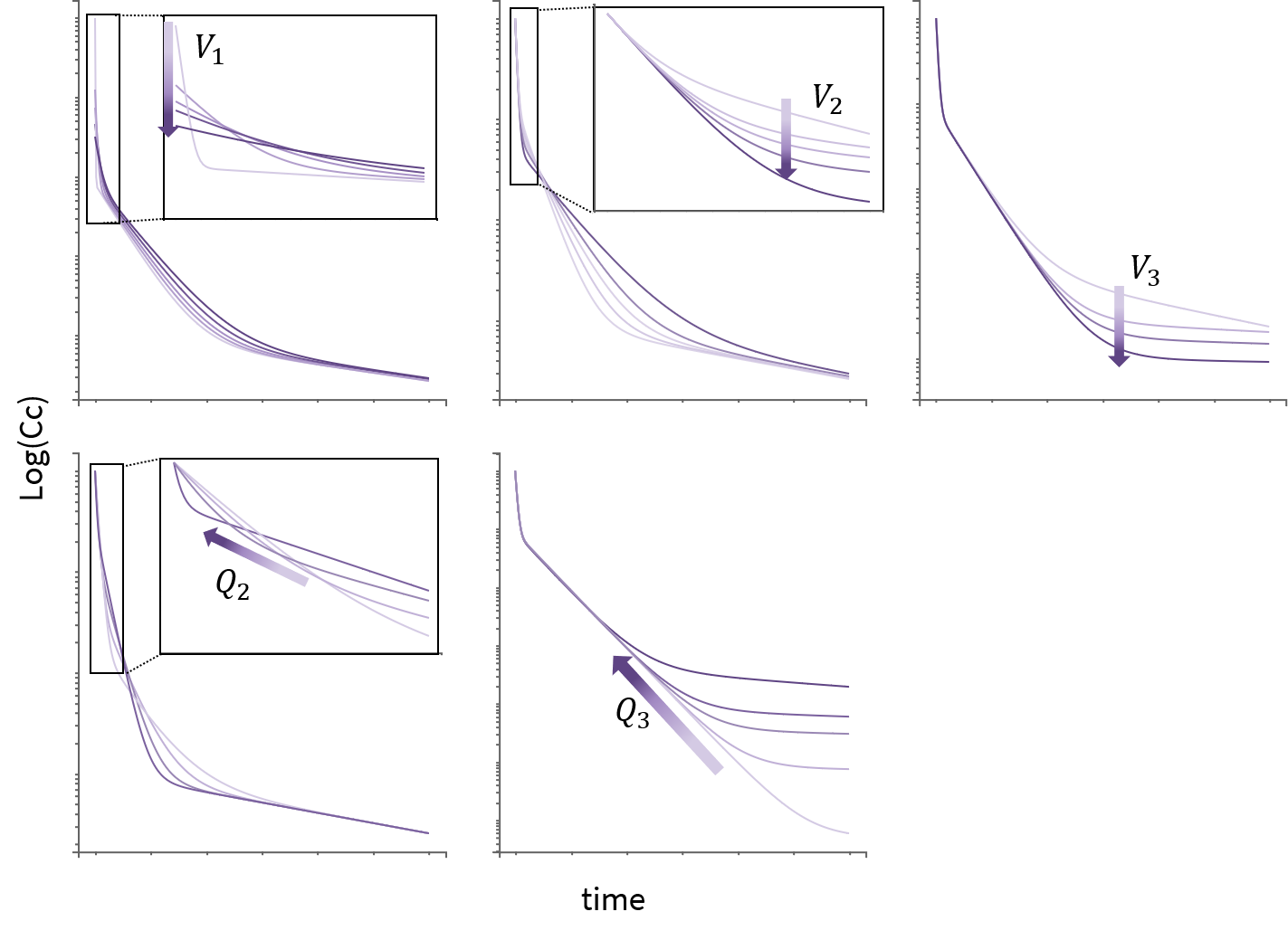
Elimination

The elimination rate denoted in the previous section as El can be either a linear rate involving the clearance Cl, or a Michaelis Menten rate involving the constants Km and Vm. Another possible parameterization for the linear rate is using the elimination rate k=Cl/V. To visualize the difference in the response, we show below the response of a 1-compartment model to a bolus in the two cases.