Categorical data models

Details on the different types of models for categorical data that can be used in Simulx and their syntax are given here: Categorical observation model

On the current page, we show an example from the Simulx demos and explains the format of simulated categorical data.

Ordered categorical data with covariate effect

7.2.categorical/categorical.smlx (model = ‘categorical_model.txt’)

In this demo, we model categorical observations, which can take seven different values. The categories are ordered and we use cumulative odds ratio to define the probability of each category in the model. The dose level of the treatment is encoded as a continuous covariate which impacts the slope parameter. Random effects are considered on the cumulative odds ratios.

CODE

[COVARIATE]
input = Dose

EQUATION:
logtDose = log(Dose/15)

[INDIVIDUAL]
input = {th0_pop, th1_pop, th2_pop, th3_pop, th4_pop, th5_pop, slope_pop, omega_slope, omega_th0, omega_th1, omega_th2, omega_th3, omega_th4, omega_th5, logtDose, beta_slope_logtDose}

DEFINITION:
th0 = {distribution=normal, typical=th0_pop, sd=omega_th0}
th1 = {distribution=logNormal, typical=th1_pop, sd=omega_th1}
th2 = {distribution=logNormal, typical=th2_pop, sd=omega_th2}
th3 = {distribution=logNormal, typical=th3_pop, sd=omega_th3}
th4 = {distribution=logNormal, typical=th4_pop, sd=omega_th4}
th5 = {distribution=logNormal, typical=th5_pop, sd=omega_th5}
slope = {distribution=logNormal, typical=slope_pop, covariate=logtDose, coefficient=beta_slope_logtDose, sd=omega_slope}

[LONGITUDINAL]
input = {th0, th1, th2, th3, th4, th5, slope}

EQUATION:
lgp0 = slope*t + th0
lgp1 = slope*t + th0 + th1
lgp2 = slope*t + th0 + th1 + th2
lgp3 = slope*t + th0 + th1 + th2 + th3
lgp4 = slope*t + th0 + th1 + th2 + th3 + th4
lgp5 = slope*t + th0 + th1 + th2 + th3 + th4 + th5

DEFINITION:
level = {type = categorical, categories = {0, 1, 2, 3, 4, 5, 6}
  logit(P(level<=0)) = lgp0
  logit(P(level<=1)) = lgp1
  logit(P(level<=2)) = lgp2
  logit(P(level<=3)) = lgp3
  logit(P(level<=4)) = lgp4
  logit(P(level<=5)) = lgp5
}

OUTPUT:
output = level

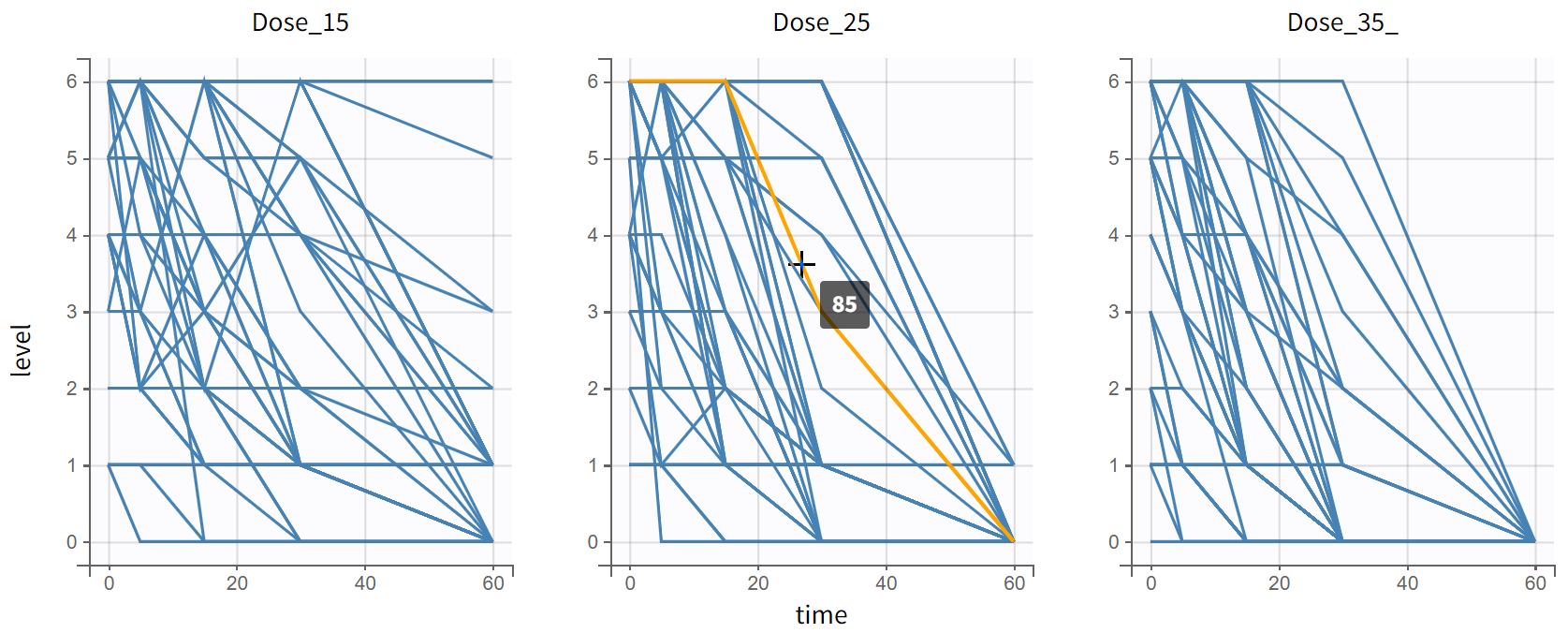
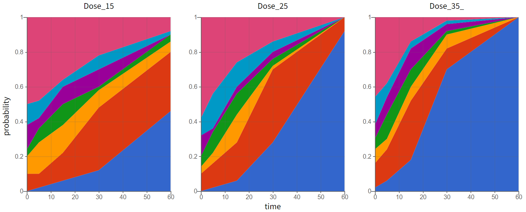
The model is simulated with 3 groups of 50 subjects with different dose levels. The simulations are displayed as individual evolution of categories over time in the Individual output plot:

and as the time evolution of probabilities of different categories in the Output distribution plot:

Formatting of categorical data in the MonolixSuite

After simulating a categorical model in Simulx, the simulated dataset can be exported. This section describes the standard format for categorical data used in the MonolixSuite.

Column-types used to define responses

https://www.youtube.com/watch?v=ZG7LhmApb_s

In case of categorical data, the observations at each time point can only take values in a fixed and finite set of nominal categories. In the data set, the output categories must be coded as consecutive integers.

Examples

Basic example:

CODE

One can see the respiratory status data set and the warfarin data set in the Monolix documentation for example for more practical examples on a categorical and a joint continuous and categorical data set respectively.