
Exposure-response analysis is an important tool for guiding clinical trial decisions, in particular dose selection and justification. It allows us to determine the relationship between the drug exposure and the drug effect, whether the effect is therapeutic or toxic. The first step of this process: calculating exposure metrics. These metrics help us describe the drug’s presence in the body - how much, how long and how it changes - and are essential for exposure-response analysis.
Link to download materials from the Feature of the Week Video: download
Some of the most common exposure metrics include:
-
Cmax, that is the peak concentration of the drug in the body, and
-
AUC, or area under the concentration curve, which reflects overall drug exposure.
For multi-dose regimens, we also calculate:
-
partial AUC, which is the AUC over a specific time interval, like between two doses or daily; and
-
C trough which is the minimum concentration before the next dose.
Metrics at steady state, such as Cmax and average steady-state concentrations, are also frequently used. These metrics represent the drug’s equilibrium, where the amount entering and leaving the body is balanced. This makes them especially useful for assessing long-term drug effects.
Exposure-response workflow:
First we built a PK model in Monolix. Then, we export this model to Simulx to calculate exposures. We can calculate exposures directly in Simulx, or simulate time-concentration curves and calculate exposures outside of Simulx using tools like R. Finally, we merge the exposure metrics with PD data and use them to build the exposure-response model in Monolix.
Example Case Study:
Dataset for a rug targeting PCSK9 to lower the cholesterol levels in the blood. PK data is the drug concentration over time and response data is the change from baseline in LDLc levels. There are 50 individuals who received 12 doses - one dose every 2 weeks over a six months period. Sampling is dense after the first dose, but for the rest of the study, we mostly have trough samples. At 6 months the drug concentration is at steady state.
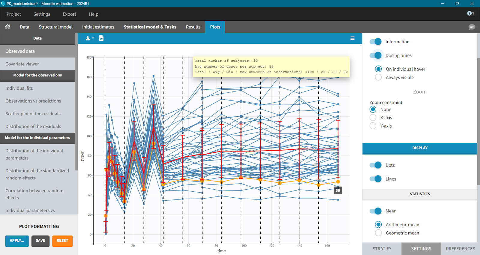
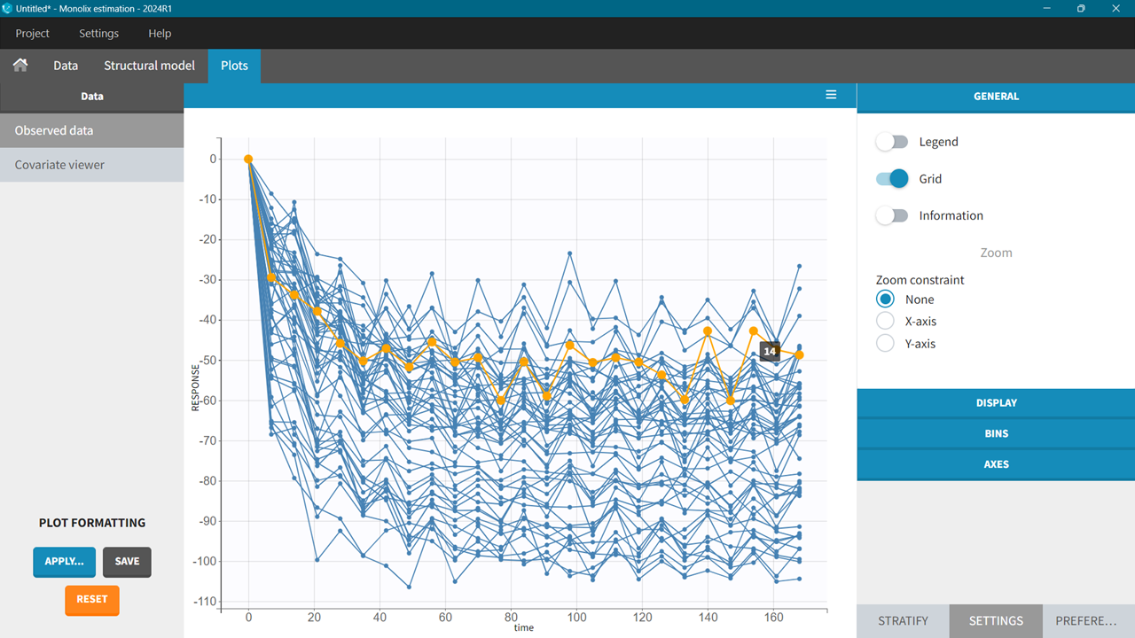
The response data in this study was also collected up to 6 months. In the following examples only subsets of this dataset will be used to explain the workflows of exposure calculation.
Exposure metrics in a single time interval
Consider that there is only one response value per individual at time 168 days and the goal is to link it with the exposures at steady state. To be sure that steady-state has been reached for all individuals, the steady state will correspond to the inter-dose interval after the last dose. Cmax, Ctrough and Cavg at steady state can be easily calculated using post-processing in Simulx’s outcomes and endpoints module.
Steps Cmax, Ctrough, Cavg:
-
Export the Monolix project with a PK model and results to Simulx. The model, parameters and treatment information will be imported.
-
In the simulation tab: switch the parameter from mlx_pop to mlx_EBEs to simulate the individuals from the original study, not a new population. Note that mlx_Adm is selected by default, which allows to re-simulate the original treatment regimen.
-
Define a new output element using model prediction of the drug concentration on a regular time grid covering the interval from 154 to 168, which corresponds to two weeks (it’s one inter-dose interval after the last dose). Rename this output element, e.g. ConcSs
-
Add new output to the simulation scenario.
-
Create outcomes based on this new output element. For Cmax, select “max value per id” as the post-processing option; for Ctrough choose “last value per id”; for average concentration use the “average value per id” option.
Steps AUC:
For AUC, the calculation requires a few additional steps, as it’s not directly available in the post-processing menu. To compute AUC in Simulx, add its definition to the model via the “additional lines” option. For cumulative AUC:
AUC_0 = 0
ddt_AUC = concentration_variable
This integrates the concentration profile from the start to a defined time point.
-
To compute AUC between two specific time points t1 and t2, use an “if/else” statement that calculates AUC from 0 to t1 and from 0 to t2. The partial AUC for the interval from t1 to t2 is simply the difference between these two values. In this example, t1=154 and t2=168.
Reminder Mlxtran syntax: If/else statement cannot contain ODEs equations. Define an intermediate variable, e.g. dAUCt1, and use it as the “right hand side” of an ODE.
t1 = 154
t2 = 168
AUCt1_0 = 0
if(t < t1)
   dAUCt1 = concentration_variable
else
   dAUCt1 = 0
end
ddt_AUCt1 = dAUCt1

AUCt2_0 = 0
if(t < t2)
   dAUCt2 = concentration_variable
else
   dAUCt2 = 0
end
ddt_AUCt2 = dAUCt2

AUC168 = AUCt2 - AUCt1
-
Create an output element for AUC using variables in the “intermediate outputs” menu. Instead of using a full time grid, use the manual method and extract the value only at t=168 to reduce computational cost.
-
Add the new output to the simulation.
-
Create an outcome for AUC - no post-processing is required but with an outcome equal to the output all the metrics are in the same result file.
Once the setup is complete, run simulation and outcomes and endpoints tasks. The results include dedicated plots for each outcome and are also presented in outcome tables. They are also saved in the output files in the result folder and can be used to merge them with the response data.
Note: You can add several partial AUC in this way, for example AUC on day 1 and day 3. It requires writing the code for each partial AUC, so if you need more than a few values, it is easier to simulate the concentration profiles on a dense time grid and calculate AUCs as a post-processing outside Simulx – see the section for inter-dose/daily AUC calculations.
Merge exposure metrics with response data via data formatting module.
Data formatting module in Monolix allows to add information from external files to a dataset for analysis without modifying the original dataset. There are two important rules:
-
The file you want to add can have only one value per individual, e.g. constant in time exposure metrics at steady state.
-
The response dataset and files with exposure metrics must have
-
the same number of individuals
-
the same subject identifiers in the column ID,
-
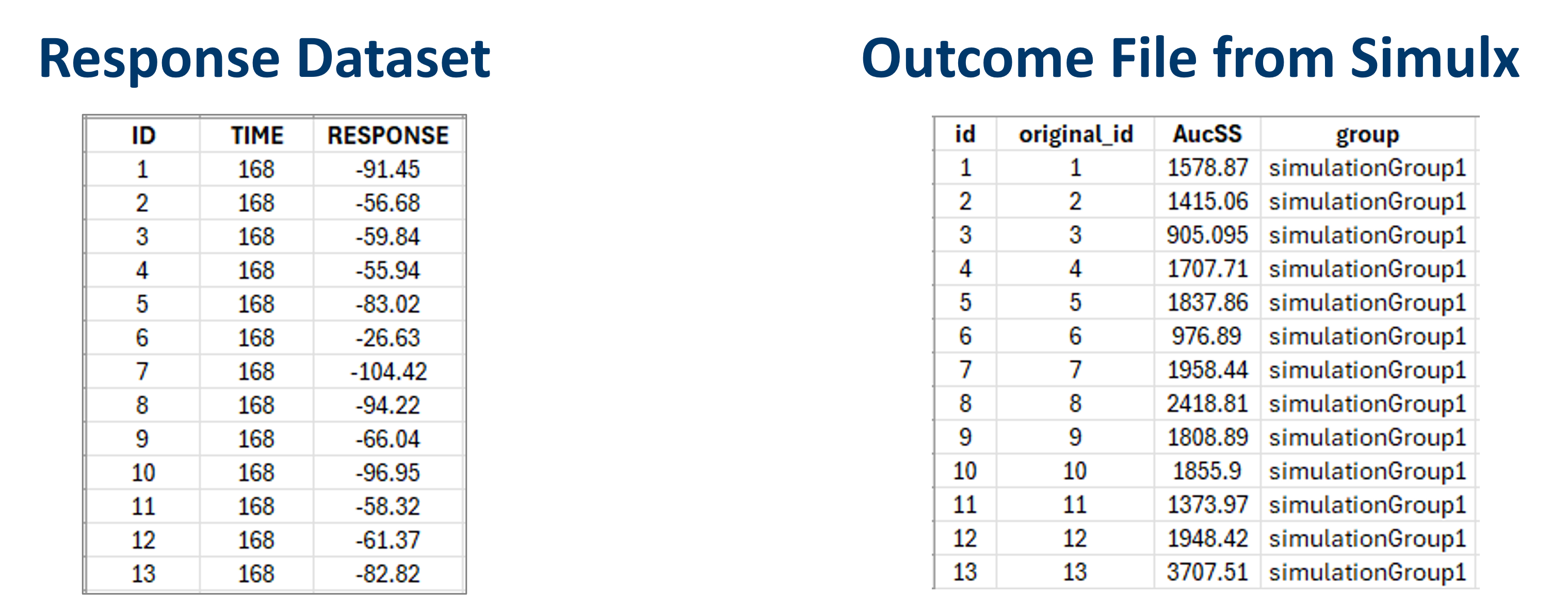
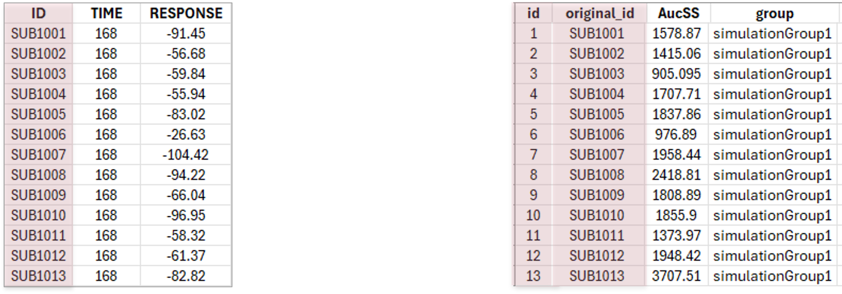
When it’s not the case - ID in a response dataset is not an integer from 1 to N, but is a custom number or a string - Simulx outcomes files cannot be merged directly in data formatting (column ID in the response dataset will be different from the column id in the outcome file).
But Simulx output files have two columns with id. Simple “id” header is for simulated ids - automatic sequential integer numbers for simulated subjects. Column with “original_id” includes specific identifiers used in simulation elements, for example in a table of individual treatments, or a table of individual parameters. The original ids are reported in the outcome result files or as a separate file.
To use data formatting in this case, modify the outcome files outside Monolix: remove the column with simulated ids and rename the column header from original-id to id.
Exposure metrics in two (or more but small number) time intervals
In this case the response dataset has two measurements per individual at the end of the first dose interval,
and at steady state.
When calculating exposure metrics over more than one time interval, but not too many intervals, the process is straightforward. Simply add a new output element in Simulx with the corresponding time limits.
In this case, if the output as the steady state is already present (from the previous example) add new output from 0 to 14 and create new outcomes as in the previous example. The same is for AUC calculation. Add the computation of AUC for additional time intervals, define output elements and add new outcomes.
When there are several exposure metric values over time, as in this example, merge the results with the response dataset cannot be done with the data formatting module in Monolix. To handle this, use an R script (example to download on top of the page) that merges data from multiple files in the Simulx “Endpoints” results folder into a single file that includes response data.
Note that exposure metrics may be available at time points where no response measurements are present. In this case, you can leave “dot” in the observation column. Conversely, if there are response measurements without corresponding exposure values. Monolix can handle this automatically by applying either a last carried forward or linear interpolation method for the missing exposure values.
Exposure metrics over several intervals (e.g. inter-dose, daily)
To calculate exposures for many intervals, such as each inter-dose intervals over a long period, daily exposures, or weekly exposures using a script in R is more efficient and flexible than doing it manually in Simulx, as in the previous example.
Steps:
-
Use a PK model built in Monolix to simulate in Simulx a concentration profiles and AUC on a fine grid covering the observation period of interest (note: previously we used Simulx to calculate directly exposure metrics)
-
Read the results in R, and calculate exposure metrics and merge them with the response data.
This method is highly flexible. It allows to define the interval lengths, the number of intervals and use individual specific intervals if needed.
After running the simulation in Simulx, use an R-script (example to download on top of the page) to calculate metrics for custom time intervals and merge then with PD data.
Note: You can calculate AUC directly in Simulx using the same approach as in previous examples. While it’s possible to calculate AUC in R, Simulx uses an ode solver and efficient C++ code. It can provide greater accuracy and efficiency than for example the trapezoidal rule in R.
Using lixoftConnectors you can automatize the whole process of building and running a simulation, exporting simulated data and using it for the post-processing.
Exposure - response analysis for a new scenario
In these three examples exposure metrics are calculated based on the original design and individuals from the original study. However, this workflow can be extended to simulate new scenarios. This procedure must be done at two stages:
-
Create a Simulx project with the PK model and simulate PK time-concentration profiles of the new scenario and calculate exposures.
-
Use the exposure-response model in a second Simulx project. Here exposures are treated as regressors, defined using external files generated during the first simulation.