plotVpc

Usage

plotVpc(
  obsName = NULL,
  eventPlot = NULL,
  settings = list(),
  preferences = list(),
  stratify = list()
)

Arguments

obsName

(character) Name of the observation (in dataset header). By default the first observation is considered.

eventPlot

(character) Display Survival function ("survivalFunction") or average number of event ("averageEventNumber) (default "survivalFunction"). For event data only.

settings

a list of optional settings:

• level (integer) level for prediction intervals computation (default 90). For continuous and discrete data only.

• higherPercentile (integer) Higher percentile for empirical and predicted percentiles computation (default 90). For continuous and event data only.

• useCorrpred (logical) if TRUE, pcVPC are computed using Uppsala prediction correction (default FALSE). For continuous data only.

• useCensored (logical) Choose to use BLQ data (TRUE) or to ignore it (FALSE) (default TRUE). For continuous data only.

• censoring (character) BLQ data can be simulated ('simulated'), or can be equal to the limit of quantification ('loq') (default 'simulated'). For continuous data only.

• timeAfterLastDose (logical) display observations only after last dose (default FALSE) For continuous and discrete data with dose information only.

• xvariable (character) choose plot abscissa if available, one of "time", "nominalTime" or a regressor name (default "time") For event data, plot against regressor value is not available.

• nbDataPoints (integer) Number of data point in event time grid (default 100) For event data only.

• xBinsSettings a list of optional settings for time axis binning For continuous and discrete data only

  • criteria (character) Bining criteria, one of 'equalwidth', 'equalsize', or 'leastsquare' methods. (default leastsquare).

  • is.fixedNbBins (logical) If TRUE define a fixed number of bins, else define a range for automatic selection (default FALSE).

  • nbBins (integer) Define a fixed number of bins (default 10).

  • binRange (vector(integer, integer)) Define a range for the number of bins (default c(5, 100)).

  • nbBinData (vector(integer, integer)) Define a range for the number of data points per bin (default c(10, 200)).

• yBinsSettings a list of optional settings for y axis binning. For countable discrete data only

  • criteria (character) Binning criteria, one of 'equalwidth', 'equalsize', or 'leastsquare' methods. (default leastsquare).

  • is.fixedNbBins (logical) If TRUE define a fixed number of bins, else define a range for automatic selection (default TRUE).

  • nbBins (integer) Define a fixed number of bins (default 10).

  • binRange (vector(integer)) Define a range for the number of bins (default c(5, 100)).

  • nbBinData (vector(integer, integer)) Define a range for the number of data points per bin (default c(10, 200)).

• obs (logical) - If TRUE, Observed data is displayed as dots (default FALSE).

• cens (logical) - If TRUE, Censored data is displayed as dots (default FALSE).

• empirical (logical) - If TRUE, Empirical data is displayed (default TRUE): empirical percentiles for continuous data; empirical probability for discrete data; empirical curve for event data

• theoretical (logical) - If TRUE, median is displayed (default FALSE): median of predicted percentiles for continuous data, median of predicted probability for discrete data, median of KM curves for event data

• predInterval (logical) - If TRUE, Prediction interval is displayed (default TRUE).

• linearInterpolation (logical) - If TRUE set piece wise display for prediction intervals, else show bins as rectangular (default TRUE).

• outlierDots (logical) - If TRUE, Add red dots indicating empirical percentiles that are outside prediction intervals (default TRUE).

• outlierAreas (logical) - If TRUE Add red areas indicating empirical percentiles that are outside prediction intervals (default TRUE).

• binLimits (logical) - Add/remove vertical lines on the scatter plots to indicate the bins (default FALSE).

• legend (logical) add (TRUE) / remove (FALSE) plot legend (default FALSE).

• grid (logical) add (TRUE) / remove (FALSE) plot grid (default TRUE).

• xlog (logical) add (TRUE) / remove (FALSE) log scaling on x axis (default FALSE).

• ylog (logical) add (TRUE) / remove (FALSE) log scaling on y axis (default FALSE).

• xlab (character) label on x axis (default "Time").

• ylab (character) label on y axis (default obsName).

• ncol (integer) number of columns when facet = TRUE (default 4).

• xlim (c(double, double)) limits of the x axis.

• ylim (c(double, double)) limits of the y axis.

• fontsize (integer) Plot text font size.

• scales (character) Should scales be fixed ("fixed"), free ("free", the default), or free in one dimension ("free_x", "free_y") (default "free").

preferences

(optional) preferences for plot display, run getPlotPreferences("plotVpc") to check available displays.

stratify

List with the stratification arguments:

• groups - Definition of stratification groups. By default, stratification groups are already defined as one group for each category for categorical covariates, and two groups of equal number of individuals for continuous covariates. To redefine groups, for each covariate to redefine, specify a list with:

  name	character	covariate name (e.g "AGE")
  definition	(vector(continuous) || list>(categorical))	For continuous covariates, vector of break values (e.g c(35, 65)). For categorical covariates, groups of categories as a list of vectors(e.g list(c("study101"), c("study201","study202")))

• split (vector) - Vector of covariates used to split (i.e facet) the plot (by default no split is applied). For instance c("FORM","AGE").

• filter (list< list> >) - List of pairs containing a covariate name and the vector of indexes or categories (for categorical covariates) of the groups to keep (by default no filtering is applied). For instance, list("AGE",c(1,3)) to keep the individuals belonging to the first and third age group, according to the definition in groups. For instance, list("FORM","ref") using the category name for categorical covariates.

• color (vector) - Vector of covariates used for coloring (by default no coloring is applied). For instance c("FORM","AGE").

• colors - Vector of colors to use when color argument is used. Takes precedence over colors defined in preferences. For instance c("#ebecf0","#cdced1","#97989c").

Value

a ggplot2 object

See also

Examples

R

  initializeLixoftConnectors(software = "monolix")

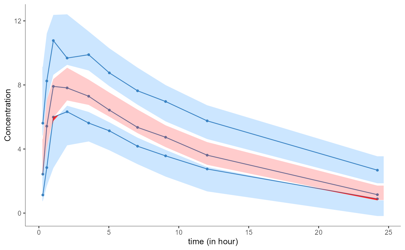
  # continuous data
  project <- file.path(getDemoPath(), "1.creating_and_using_models",
                       "1.1.libraries_of_models", "theophylline_project.mlxtran")
  loadProject(project)
  runPopulationParameterEstimation()
  plotVpc(obsName = "CONC",
          settings = list(outlierDots = FALSE, grid = FALSE,
                          ylab = "Concentration", xlab = "time (in hour)"))

R

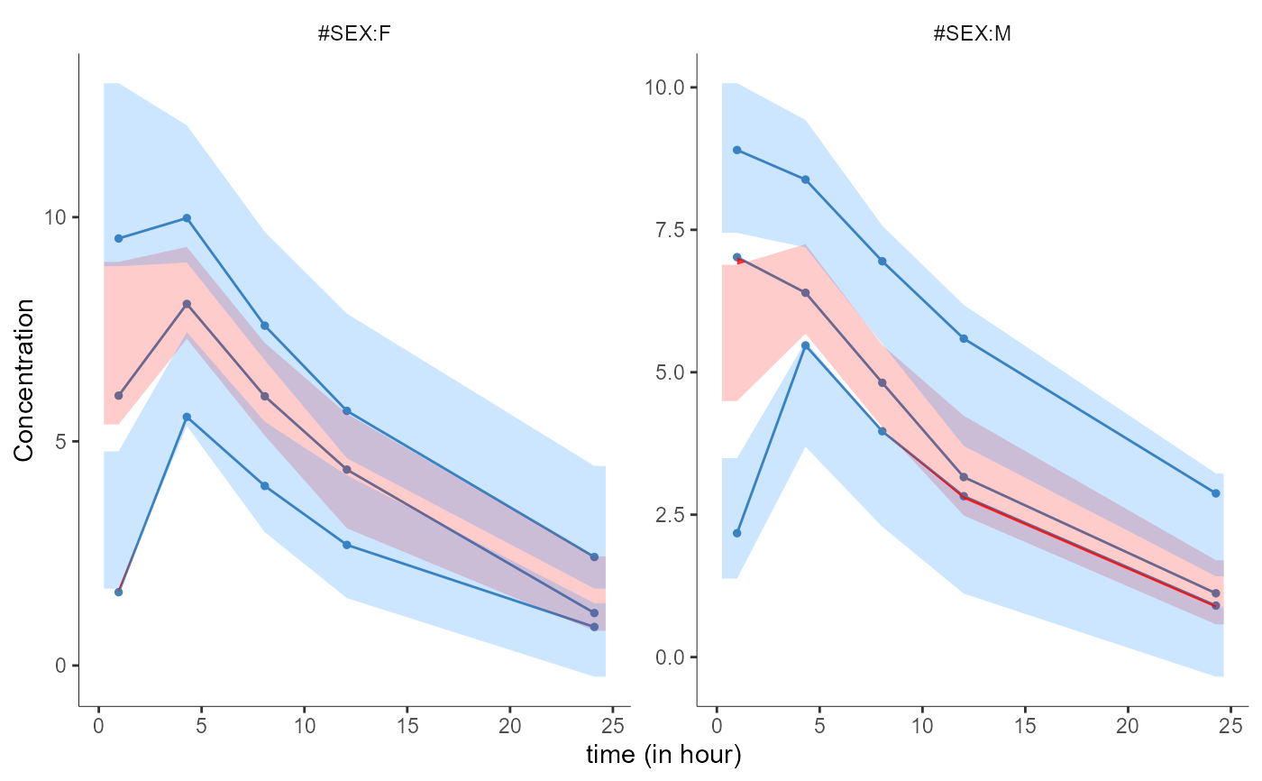
  plotVpc(obsName = "CONC",
          settings = list(outlierDots = FALSE, grid = FALSE,
                          ylab = "Concentration", xlab = "time (in hour)"),
          stratify = list(split = "SEX"))

R

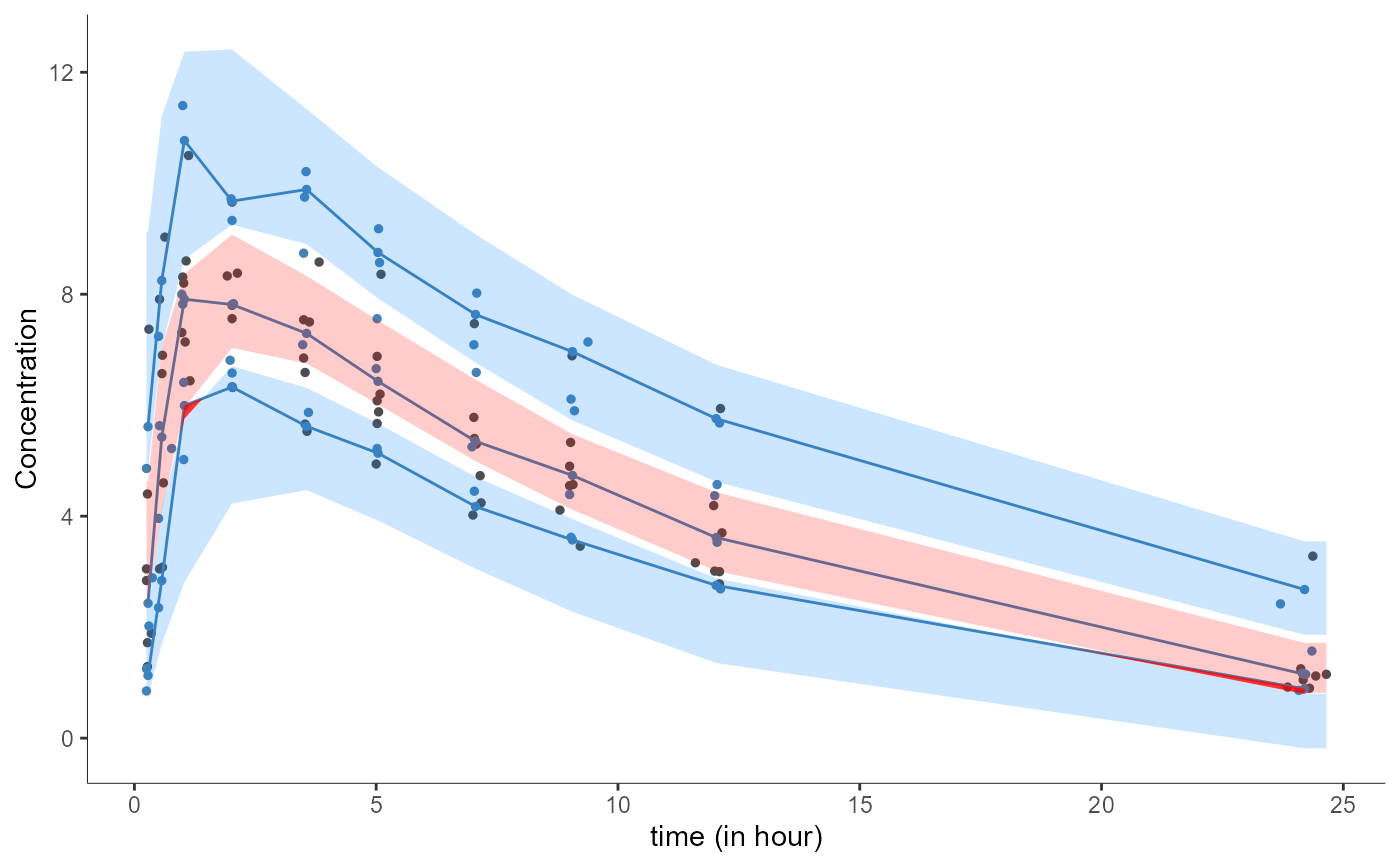
  plotVpc(obsName = "CONC",
          settings = list(outlierDots = FALSE, grid = FALSE, obs = TRUE,
                          ylab = "Concentration", xlab = "time (in hour)"),
          stratify = list(color = "SEX"))

R

                         
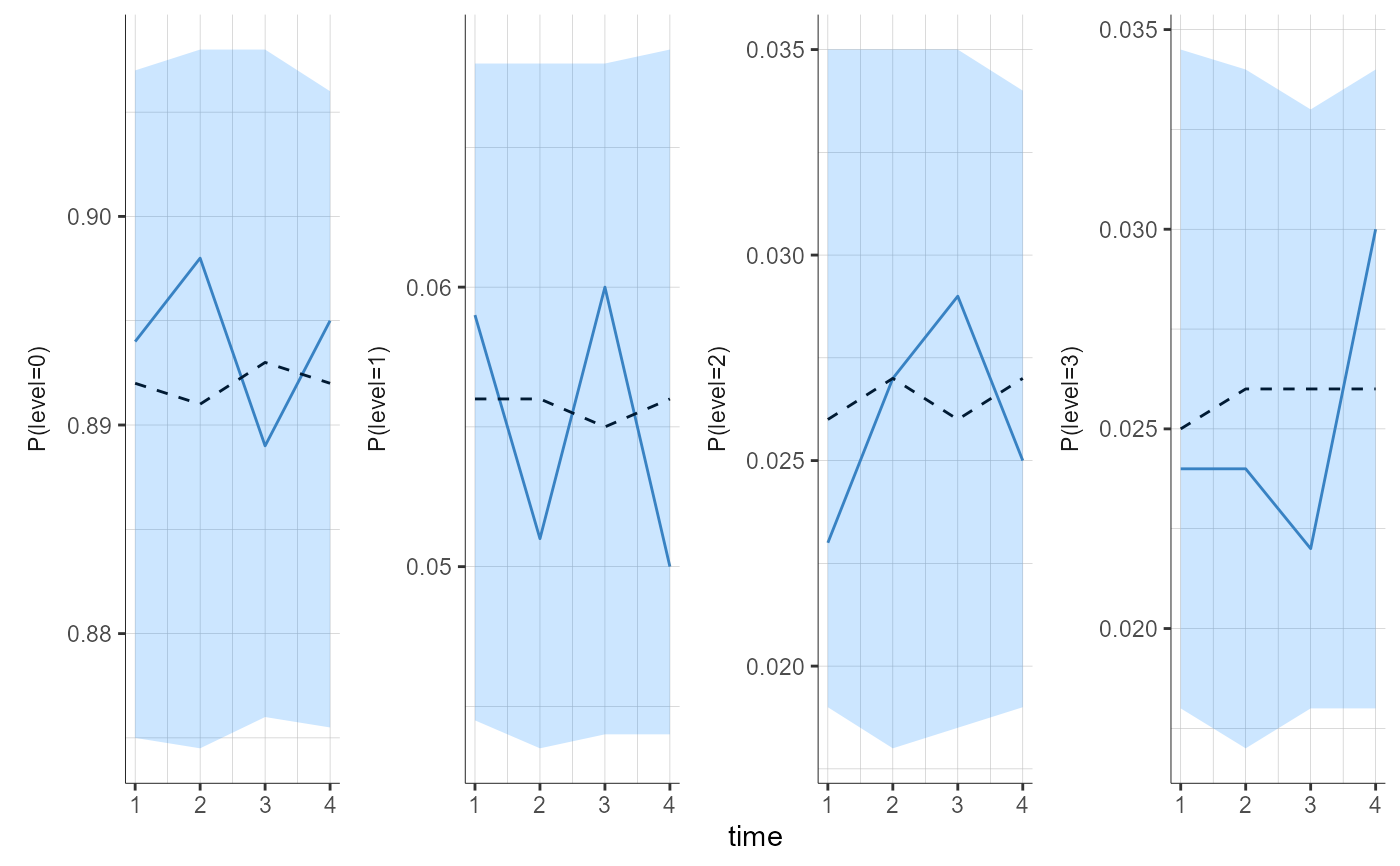
  # categorical data
  project <- file.path(getDemoPath(), "3.models_for_noncontinuous_outcomes",
                       "3.1.categorical_data_model", "categorical1_project.mlxtran")
  loadProject(project)
  runPopulationParameterEstimation()
  plotVpc(obsName = "level",
          settings = list(theoretical = TRUE, outlierDots = FALSE))

R

                         
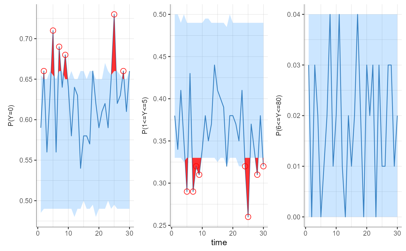
  # countable data
  project <- file.path(getDemoPath(), "3.models_for_noncontinuous_outcomes",
                       "3.2.count_data_model", "count1a_project.mlxtran")
  loadProject(project)
  runPopulationParameterEstimation()
  plotVpc(obsName = "Y")

R

               
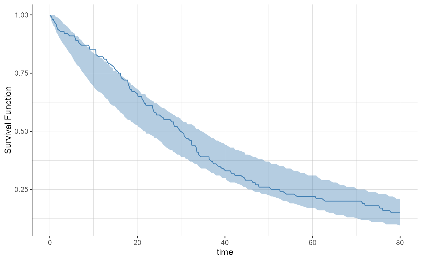
  # time to event data
  project <- file.path(getDemoPath(), "3.models_for_noncontinuous_outcomes",
                       "3.3.time_to_event_data_model", "tte1_project.mlxtran")
  loadProject(project)
  runPopulationParameterEstimation()
  plotVpc(obsName = "Event", eventPlot = "survivalFunction")

R

$body