
[Monolix] Generate Distribution of the residuals
Plot the distribution of the residuals.
Usage
plotResidualsDistribution(
  obsName = NULL,
  residuals = c("indiv", "npde"),
  plots = c("pdf", "cdf"),
  settings = list(),
  preferences = list(),
  stratify = list()
)
Arguments
obsName (character) Name of the observation (in dataset header). By default the first observation is considered. residuals (character) List of residuals to display: population residuals ("pop"), individual residuals ("indiv"), normalized prediction distribution error ("npde") (default c("indiv", "npde)). plots Type of plots: probability density distribution ("pdf"), cumulative density distribution ("cdf") (default c("pdf", "cdf")). settings List with the following settingsindivEstimate (character) Calculation of individual estimates: conditional mean ("mean"), conditional mode with EBE's ("mode"), conditional distribution ("simulated") (default "simulated"). useCensored (logical) Choose to use BLQ data (TRUE) or to ignore it (FALSE) to compute the statistics (default TRUE). For continuous data only. censoring (character) BLQ data can be simulated ('simulated'), or can be equal to the limit of quantification ('loq') (default 'simulated'). For continuous data only. legend (logical) add (TRUE) / remove (FALSE) plot legend (default FALSE). grid (logical) add (TRUE) / remove (FALSE) plot grid (default TRUE). ncol (integer) number of columns when facet = TRUE (default 4). fontsize (integer) Plot text font size. preferences (optional) preferences for plot display, run getPlotPreferences("plotResidualsDistribution") to check available displays. stratify List with the stratification arguments:groups - Definition of stratification groups. By default, stratification groups are already defined as one group for each category for categorical covariates, and two groups of equal number of individuals for continuous covariates. To redefine groups, for each covariate to redefine, specify a list with:namecharactercovariate name (e.g "AGE")definition(vector(continuous) || list>(categorical))For continuous covariates, vector of break values (e.g c(35, 65)). For categorical covariates, groups of categories as a list of vectors(e.g list(c("study101"), c("study201","study202"))) split (vector) - Vector of covariates used to split (i.e facet) the plot (by default no split is applied). For instance c("FORM","AGE"). filter (list< list> >) - List of pairs containing a covariate name and the vector of indexes or categories (for categorical covariates) of the groups to keep (by default no filtering is applied). For instance, list("AGE",c(1,3)) to keep the individuals belonging to the first and third age group, according to the definition in groups. For instance, list("FORM","ref") using the category name for categorical covariates.
Value
-
A ggplot object if one prediction type,
-
A TableGrob object if multiple plots (output of grid.arrange)
See also
getChartsData getPlotPreferences
Examples
initializeLixoftConnectors(software = "monolix")
project <- file.path(getDemoPath(), "1.creating_and_using_models",
"1.1.libraries_of_models", "theophylline_project.mlxtran")
loadProject(project)
runPopulationParameterEstimation()
runConditionalDistributionSampling()
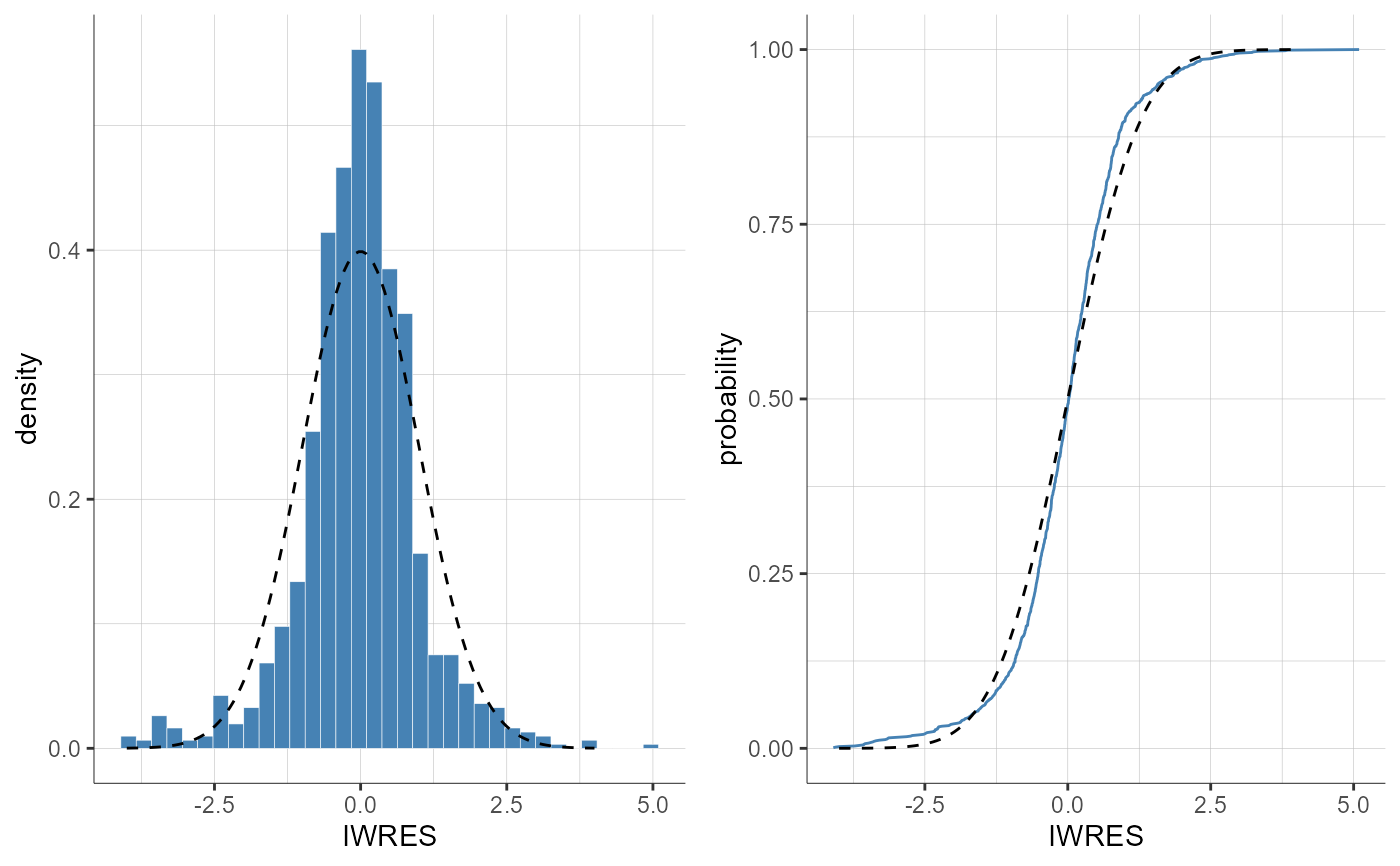
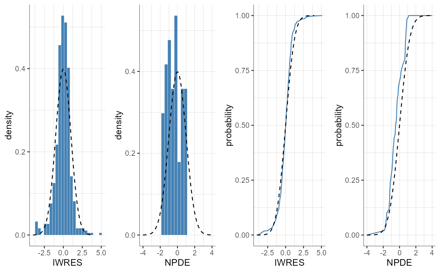
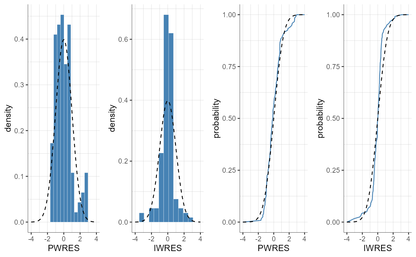
plotResidualsDistribution()

#> TableGrob (1 x 1) "arrange": 1 grobs
#>   z     cells    name            grob
#> 1 1 (1-1,1-1) arrange gtable[arrange]
  plotResidualsDistribution(residuals = "indiv", settings = list(indivEstimate = "simulated"))
#> TableGrob (1 x 1) "arrange": 1 grobs
#> z cells name grob
#> 1 1 (1-1,1-1) arrange gtable[arrange]
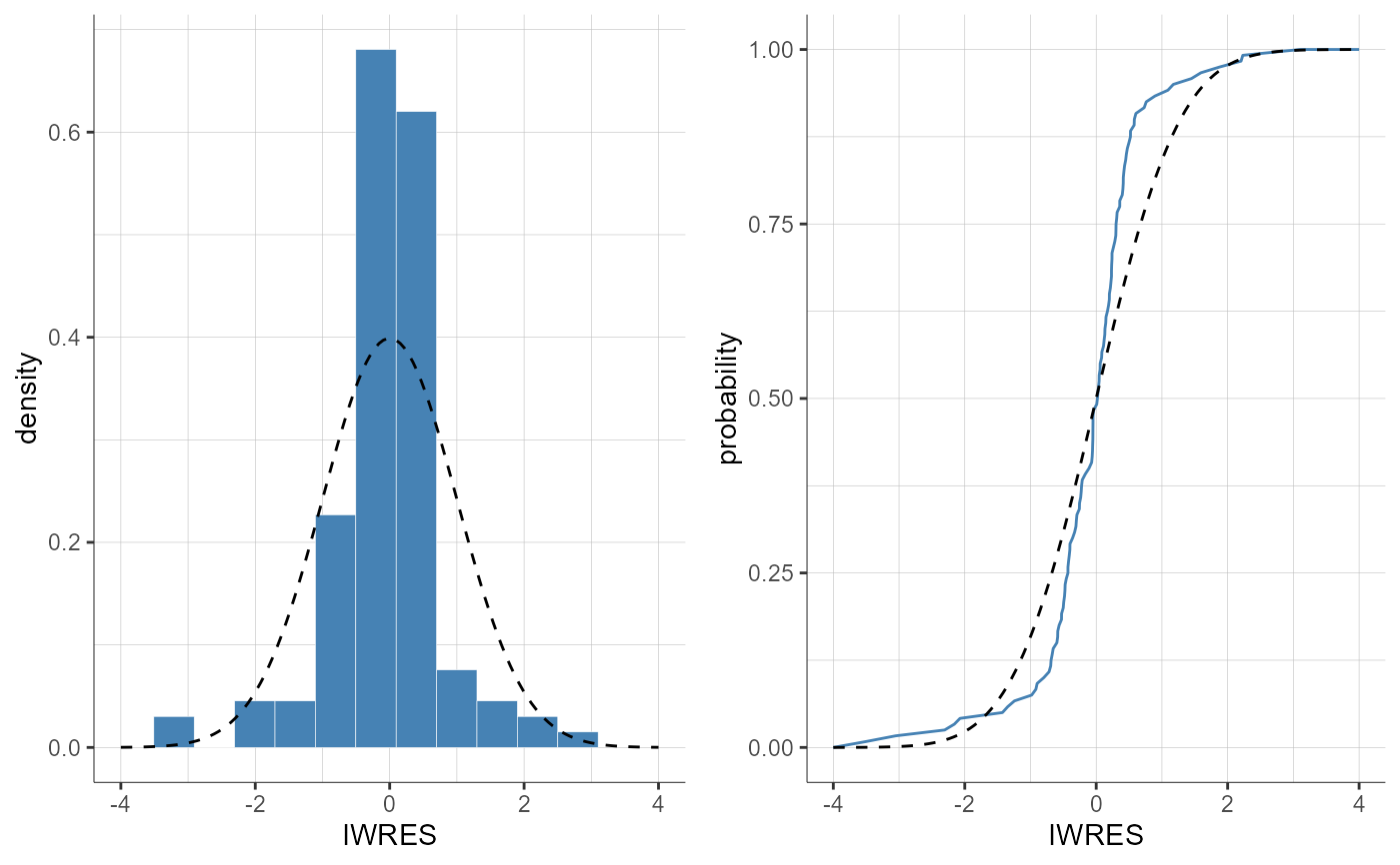
plotResidualsDistribution(residuals = "indiv", settings = list(indivEstimate = "mode"))
#> Warning: Conditional Mode Estimation was not run, individual predictions based on conditional mean computed with MCMC will be displayed instead.
#> TableGrob (1 x 1) "arrange": 1 grobs
#> z cells name grob
#> 1 1 (1-1,1-1) arrange gtable[arrange]
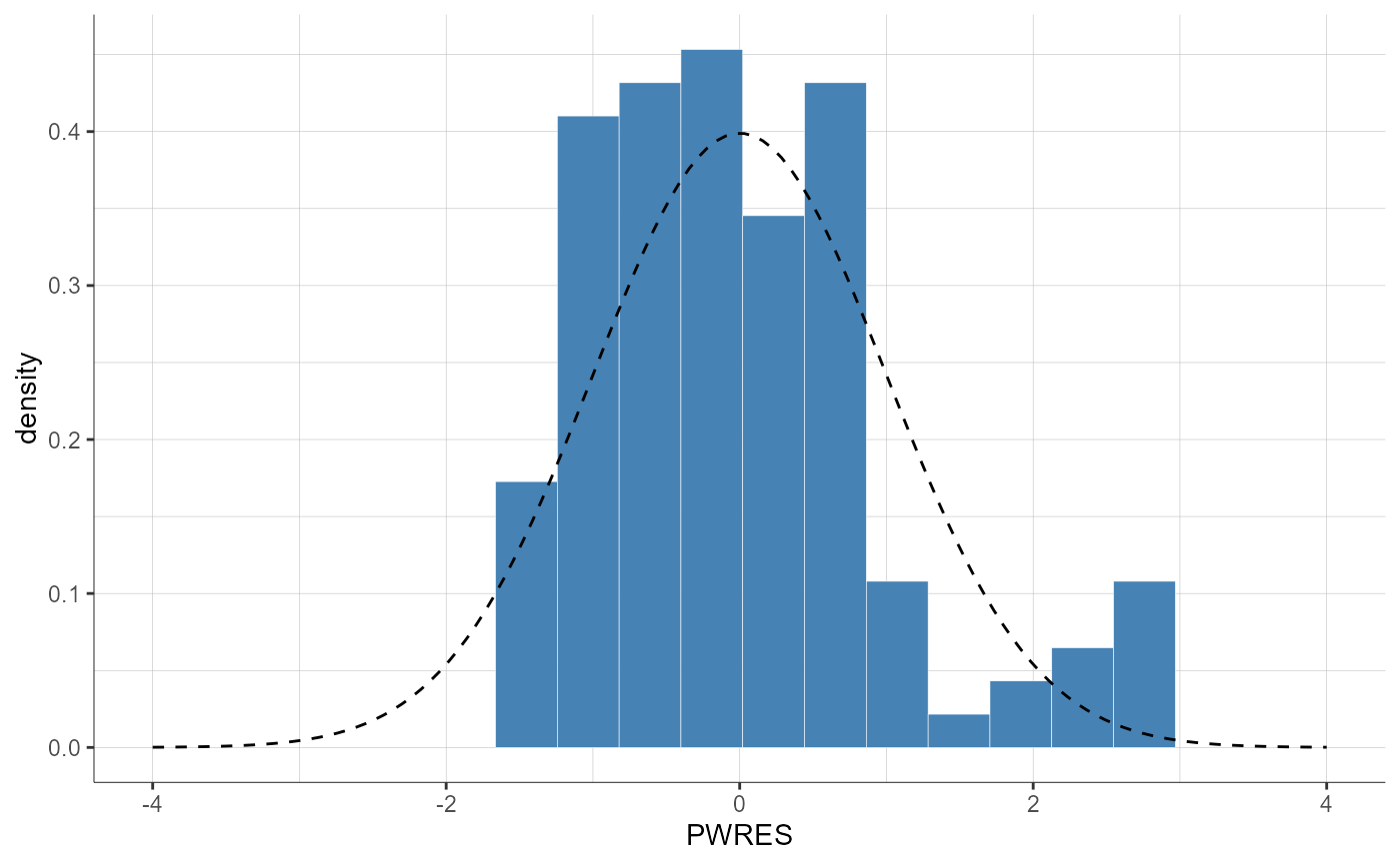
plotResidualsDistribution(residuals = "pop", plots = "pdf")
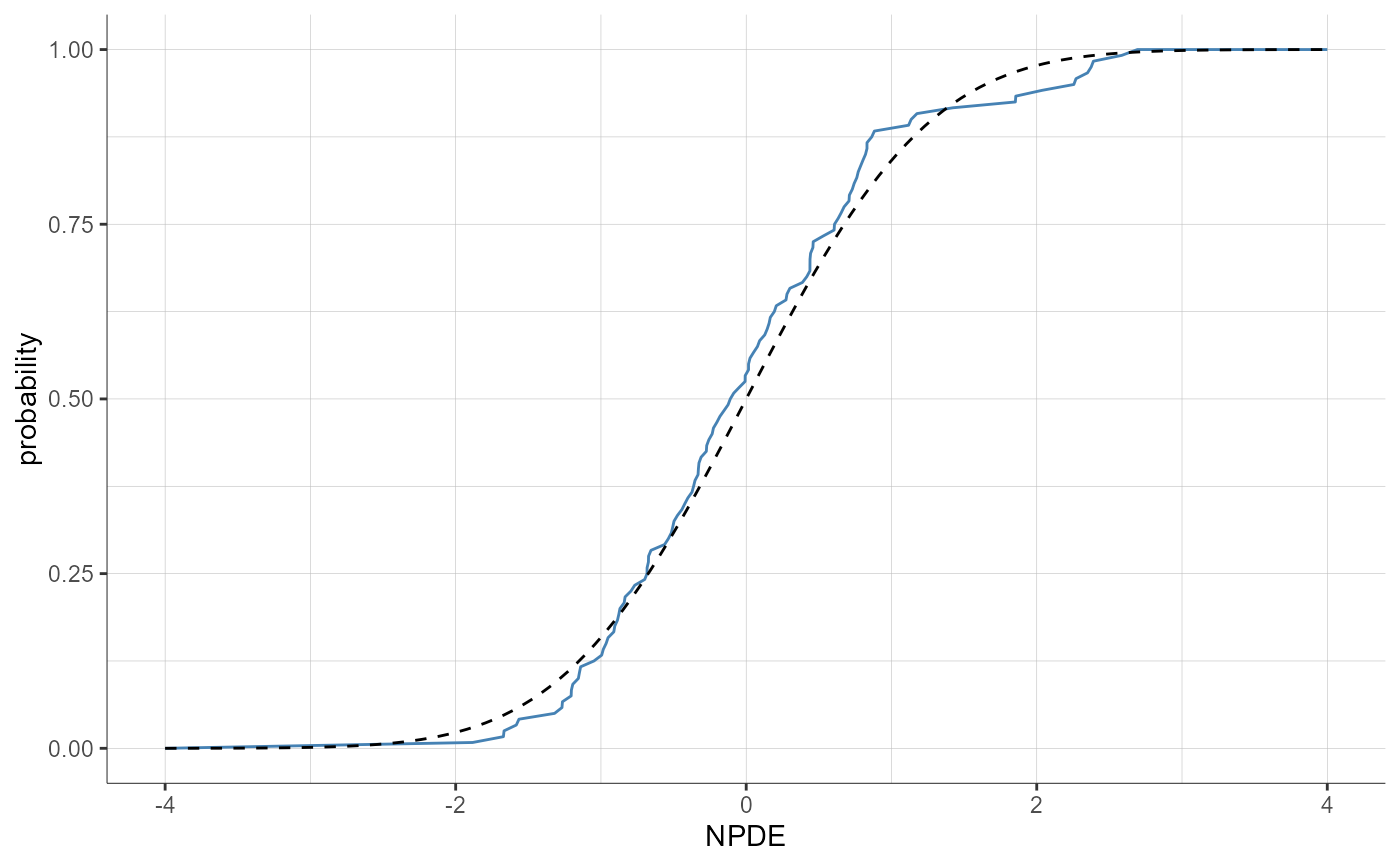
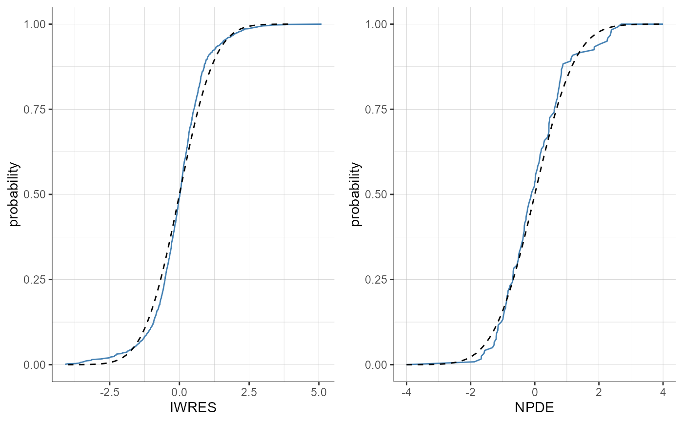
plotResidualsDistribution(residuals = "npde", plots = "cdf")
plotResidualsDistribution(stratify = list(filter=list("SEX", "F")))
#> TableGrob (1 x 1) "arrange": 1 grobs
#>   z     cells    name            grob
#> 1 1 (1-1,1-1) arrange gtable[arrange]
  plotResidualsDistribution(stratify = list(split = "WEIGHT",
                                            groups = list(name = "WEIGHT", definition = c(75))))
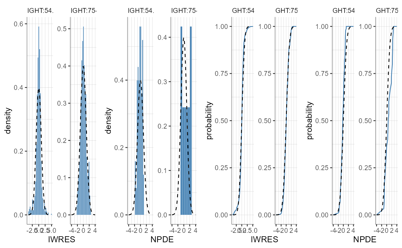
#> TableGrob (1 x 1) "arrange": 1 grobs
#>   z     cells    name            grob
#> 1 1 (1-1,1-1) arrange gtable[arrange]
  plotResidualsDistribution(residuals = "indiv", settings = list(legend = T),
                            stratify = list(split = c("SEX", "WEIGHT"),
                                            groups = list(name = "WEIGHT", definition = 70)))
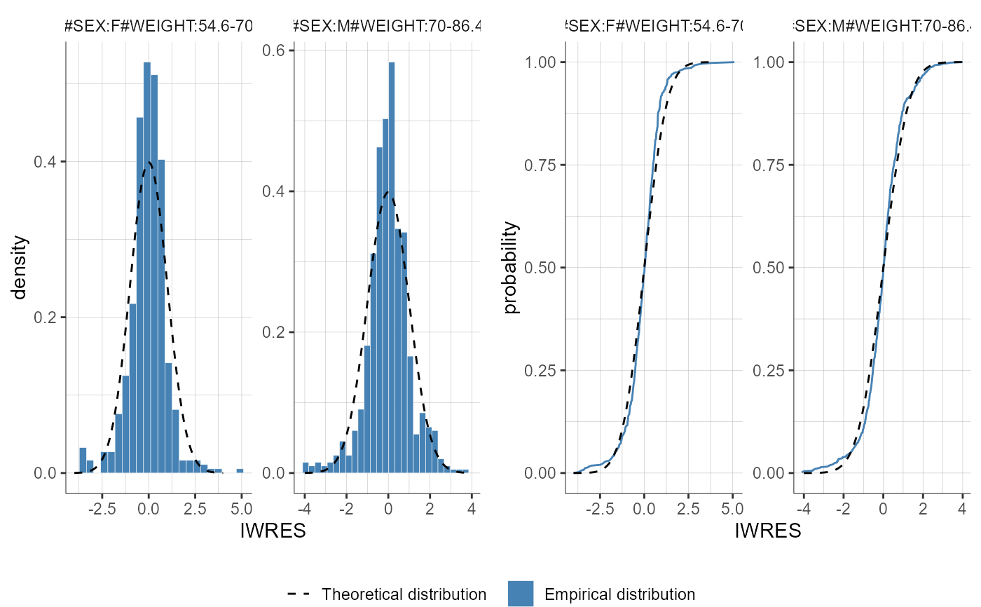
#> TableGrob (2 x 1) "arrange": 2 grobs
#>   z     cells    name              grob
#> 1 1 (1-1,1-1) arrange   gtable[arrange]
#> 2 2 (2-2,1-1) arrange gtable[guide-box]

  plotResidualsDistribution()
#> TableGrob (1 x 1) "arrange": 1 grobs
#>   z     cells    name            grob
#> 1 1 (1-1,1-1) arrange gtable[arrange]
  plotResidualsDistribution(residuals = c("indiv", "npde"), settings = list(indivEstimate = "simulated"))

#> TableGrob (1 x 1) "arrange": 1 grobs
#>   z     cells    name            grob
#> 1 1 (1-1,1-1) arrange gtable[arrange]
  plotResidualsDistribution(residuals = c("pop", "indiv"), settings = list(indivEstimate = "mode"))
#> Warning: Conditional Mode Estimation was not run, individual predictions based on conditional mean computed with MCMC will be displayed instead.
#> TableGrob (1 x 1) "arrange": 1 grobs
#>   z     cells    name            grob
#> 1 1 (1-1,1-1) arrange gtable[arrange]
  plotResidualsDistribution(plots = c("pdf", "cdf"))

#> TableGrob (1 x 1) "arrange": 1 grobs
#>   z     cells    name            grob
#> 1 1 (1-1,1-1) arrange gtable[arrange]
  plotResidualsDistribution(plots = c("cdf"))
#> TableGrob (1 x 1) "arrange": 1 grobs
#> z cells name grob
#> 1 1 (1-1,1-1) arrange gtable[arrange]
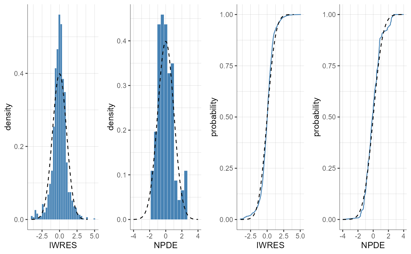
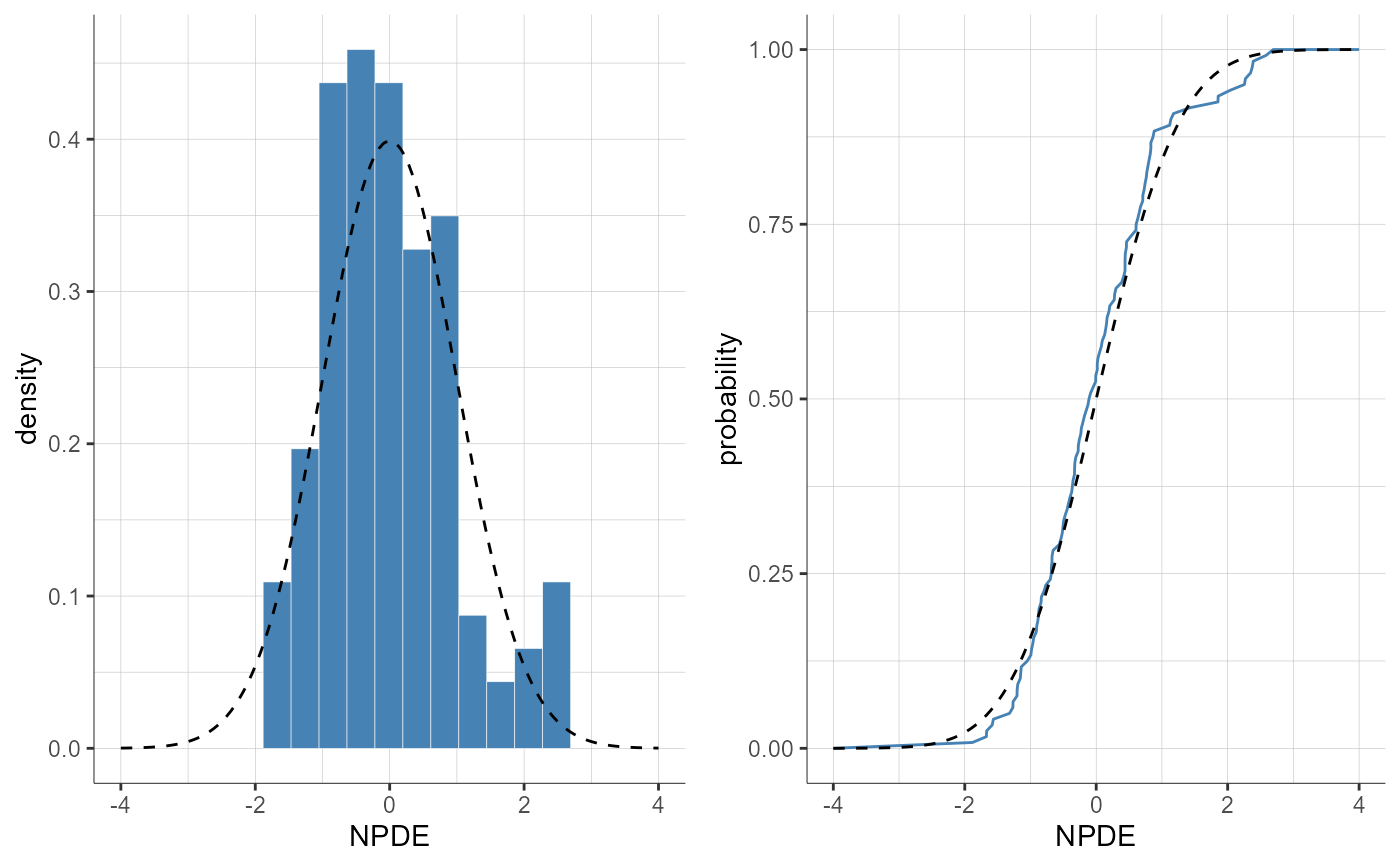
plotResidualsDistribution(residuals = "npde")
#> TableGrob (1 x 1) "arrange": 1 grobs
#>   z     cells    name            grob
#> 1 1 (1-1,1-1) arrange gtable[arrange]