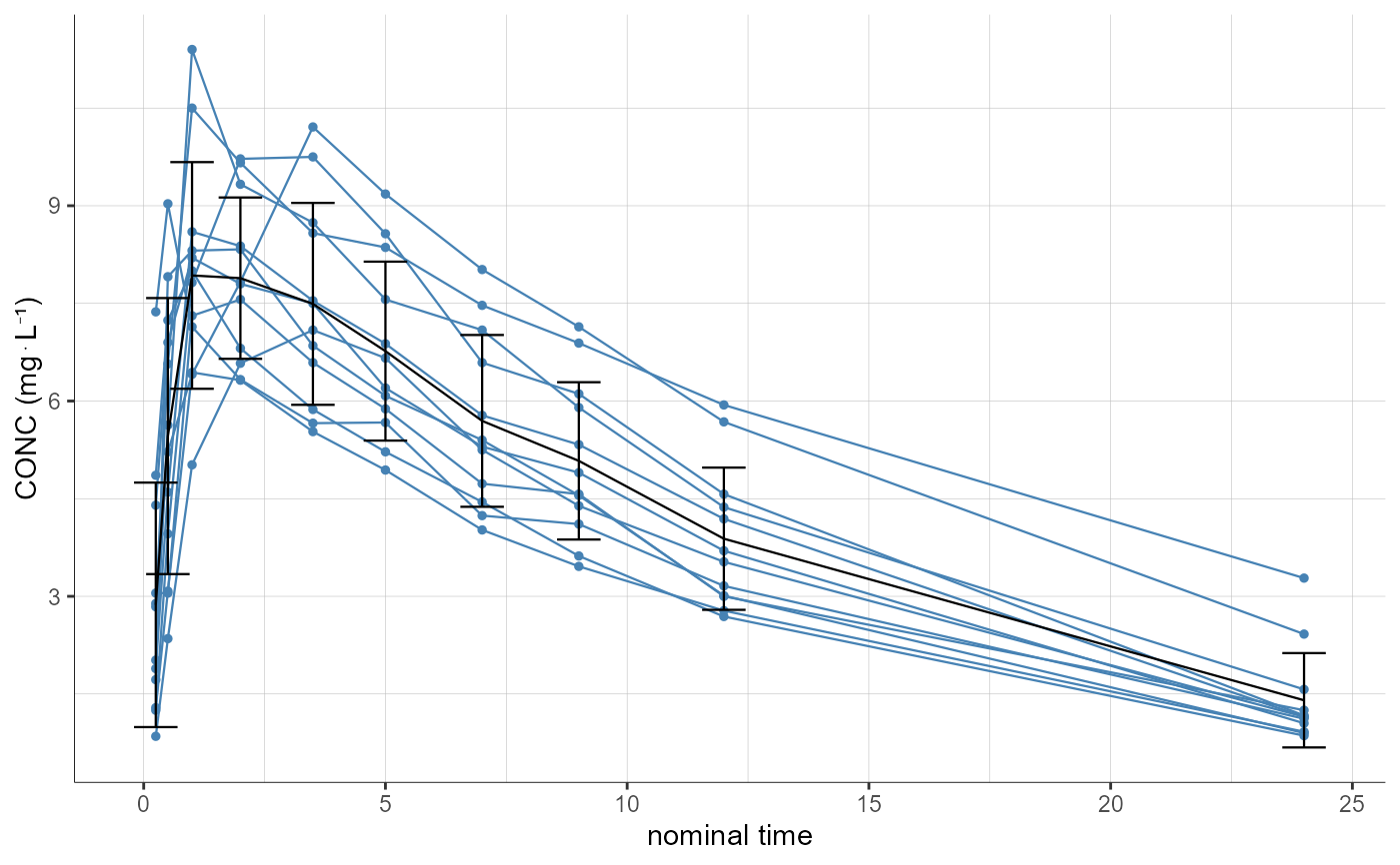
[Monolix - PKanalix] Generate Observed data plot
Plot the observed data.
Usage
plotObservedData(
  obsName = NULL,
  settings = list(),
  stratify = list(),
  preferences = list()
)
Arguments
obsName (character) Name of the observation (if several OBS ID). By default the first observation is considered. settings List with the following settings: [CONTINUOUS - DISCRETE] Settings specific to continuous and discrete datadots (logical) - If TRUE individual observations are displayed as dots (default TRUE). lines (logical) - If TRUE individual observations are displayed as lines (default TRUE). mean (logical) - If TRUE mean of observations is displayed (default FALSE for Monolix, TRUE for PKanalix). error (logical) If TRUE error bar is displayed (default FALSE for Monolix, TRUE for PKanalix). meanMethod (character) - When mean is set to TRUE, display arithmetic mean ("arithmetic") or geometric mean ("geometric"). Default value is "arithmetic". errorMethod (character) - When error is set to TRUE, display standard deviation ("standardDeviation") or standard error ("standardError"). Default value is "standardDeviation". useCensored (logical) If TRUE, use censored data to compute mean and error (default FALSE) timeAfterLastDose (logical) If TRUE, display observations as relative to the previous dose for the x-axis (default FALSE) Can be applied only for continuous and discrete data with dose information, and if xvariable is different from "regressor". xvariable (character) Choose information to use on x-axis, one of "time", "nominalTime" or a regressor name (default "time") For event data, plot against regressor value is not available. binLimits (logical) - If TRUE, bins limits are displayed as vertical lines (default FALSE). binsSettings a list of settings for time axis binning for observation statistics computation:criteria (character) - Binning criteria, one of 'equalwidth', 'equalsize', or 'leastsquare' methods. (default "leastsquare"). is.fixedNbBins (logical) - If TRUE, a fixed number of bins is used (see nbBins). If FALSE (default), the number of bins is optimized using binRange and nbBinData. nbBins (integer) - Number of bins (default 10). Ignored if is.fixedNbBins=FALSE. binRange (vector(integer, integer)) - Minimum and maximum number of bins when bins are optimized (default c(5, 100)). nbBinData (vector(integer, integer)) - Minimum and maximum number of data points per bin when bins are optimized (default c(10, 200) for Monolix and c(3, 200) for PKanalix). [DISCRETE] Settings specific to discrete dataplot (character) Type of plot: "continuous" (default), "stacked" or "grouped". histogramColors (vector) List of colors to use in histograms plots. [EVENT] Settings specific to event dataeventPlot - Display Survival function ("survivalFunction") or mean number of events per subject ("averageEventNumber") (default "survivalFunction"). Other settingscens (logical) - If TRUE censored data are displayed as dots (default TRUE). dosingTimes (logical) - If TRUE, dosing times are displayed as vertical lines (default FALSE). Cannot be used if timeAfterLastDose=TRUE. legend (logical) - If TRUE, plot legend is displayed (default FALSE). grid (logical) - If TRUE, plot grid is displayed (default TRUE). xlog (logical) - If TRUE, log-scale on x axis is used (default FALSE). ylog (logical) - If TRUE, log-scale on y axis is used (default FALSE). xlab (character) - Label on x axis (default "time"). ylab (character) - Label on y axis (default obsName). ncol (integer) - Number of columns when using split (default 4). xlim (c(double, double)) - Limits of the x axis. ylim (c(double, double)) - Limits of the y axis. fontsize (integer) - Font size of text elements (default 11). units (logical) - If TRUE, units are added in axis labels (default TRUE) (only available with PKanalix). scales (character) Should scales be fixed ("fixed"), free ("free", default), or free in one dimension ("free_x", "free_y"). stratify List with the stratification arguments:groups - Definition of stratification groups. By default, stratification groups are already defined as one group for each category for categorical covariates, and two groups of equal number of individuals for continuous covariates. To redefine groups, for each covariate to redefine, specify a list with:namecharactercovariate name (e.g "AGE")definition(vector(continuous) || list>(categorical))For continuous covariates, vector of break values (e.g c(35, 65)). For categorical covariates, groups of categories as a list of vectors(e.g list(c("study101"), c("study201","study202"))) split (vector) - Vector of covariates used to split (i.e facet) the plot (by default no split is applied). For instance c("FORM","AGE"). mergedSplits (logical) - When "split" is used and mean=T, should the means of the different groups be displayed on the same plot (TRUE) or on different subplots (FALSE, default). Not available for count/categorical data. When mergedSplits=T, the "color" argument is ignored and the coloring is done according to the splitted groups. filter (list< list> >) - List of pairs containing a covariate name and the vector of indexes or categories (for categorical covariates) of the groups to keep (by default no filtering is applied). For instance, list("AGE",c(1,3)) to keep the individuals belonging to the first and third age group, according to the definition in groups. For instance, list("FORM","ref") using the category name for categorical covariates. color (vector) - Vector of covariates used for coloring (by default no coloring is applied). For instance c("FORM","AGE"). colors - Vector of colors to use when color argument is used. Takes precedence over colors defined in preferences. For instance c("#ebecf0","#cdced1","#97989c"). individualSelection - Ids to display (by default the 12 first ids are displayed) defined as:indices (vector) - Indices of the individuals to display (by default, the 12 first individuals are selected). If occasions are present, all occasions of the selected individuals will be displayed. Takes precedence over ids. For instance c(5,6,10,11). isRange (logical) - If TRUE, all individuals whose index is inside [min(indices), max[indices]] are selected (FALSE by default). Forced to FALSE if ids is defined. ids (vector) - Names of the individuals to display. If occasions are present, all occasions of the selected individuals will be displayed. For instance c("101-01","101-02","101-03"). If ids are integers, can also be c(1,3,6). Ignored if indices is defined. preferences (optional) preferences for plot display, run getPlotPreferences("plotObservedData") to check available options.
Value
A ggplot object
See also
Examples
  initializeLixoftConnectors(software = "pkanalix", force=T)
  project <- paste0(getDemoPath(), "/2.case_studies/project_aPCSK9_SAD.pkx")
  loadProject(project)

  # by default, individual profiles and mean curve are displayed
  plotObservedData()
#> Warning: No shared levels found between `names(values)` of the manual scale and the
#> data's linetype values.
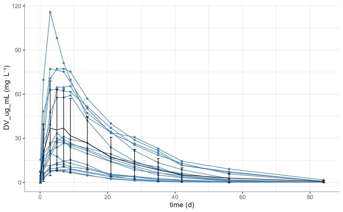
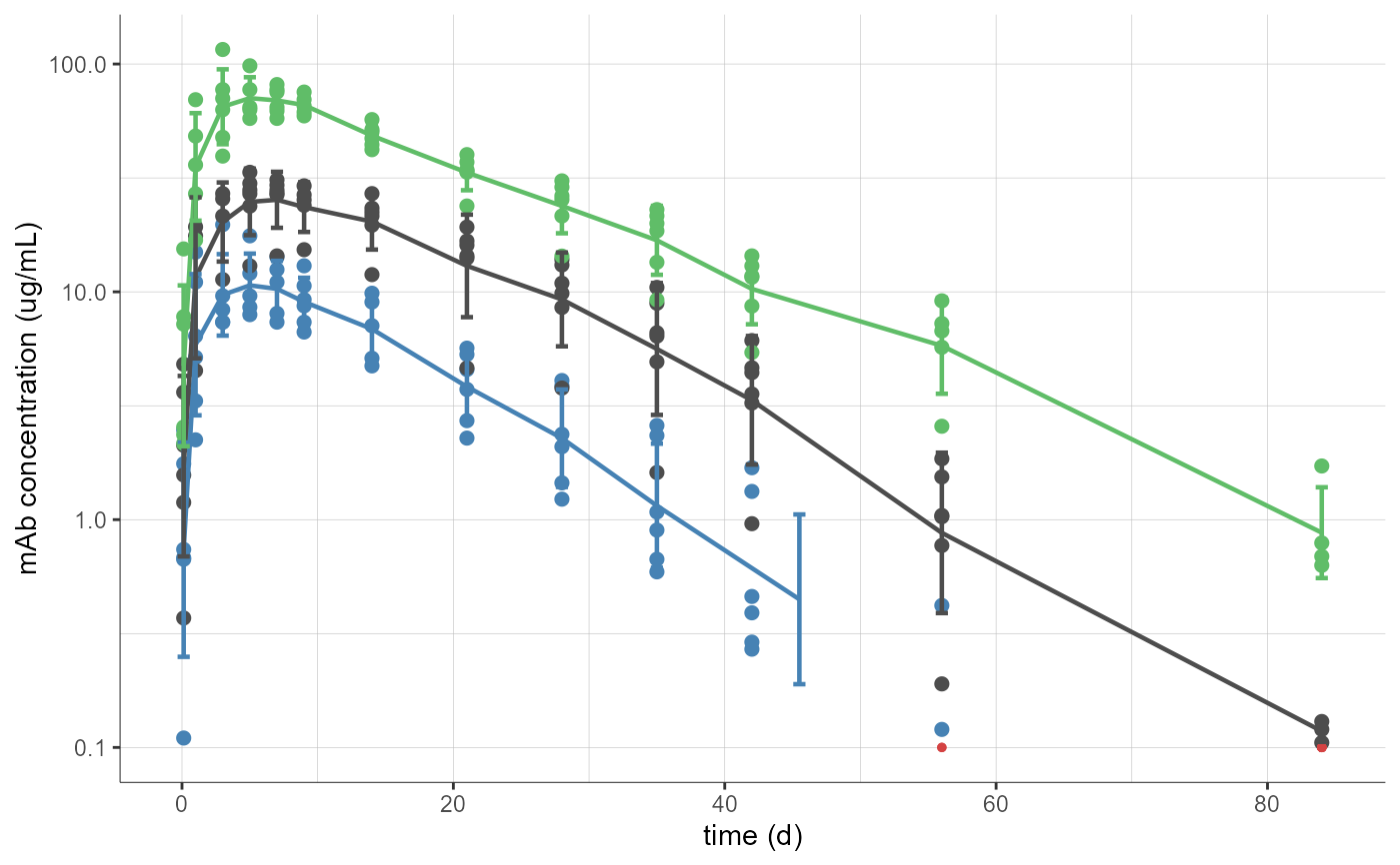
  # displaying dots and mean curve by dose group, merged on a single plot
  plotObservedData(settings=list(lines=F,
                            mean=T,
                            meanMethod="geometric",
                            ylog=T,
                            ylab="mAb concentration (ug/mL)"),
              stratify=list(split="DOSE_mg",
                            mergedSplits=T),
              preferences=list(observationStatistics=list(lineWidth=0.8),
                               obs=list(radius=2)))
#> Warning: No shared levels found between `names(values)` of the manual scale and the
#> data's linetype values.
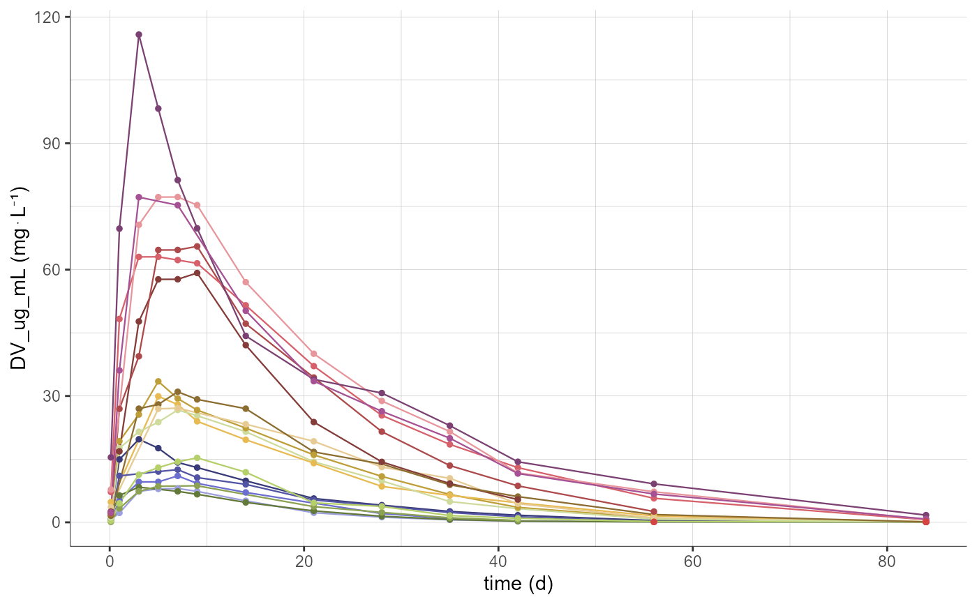
  # coloring by ID, without mean curve
  plotObservedData(settings=list(mean=F,error=F),
              stratify = list(color=c("id")))
#> Warning: No shared levels found between `names(values)` of the manual scale and the
#> data's linetype values.
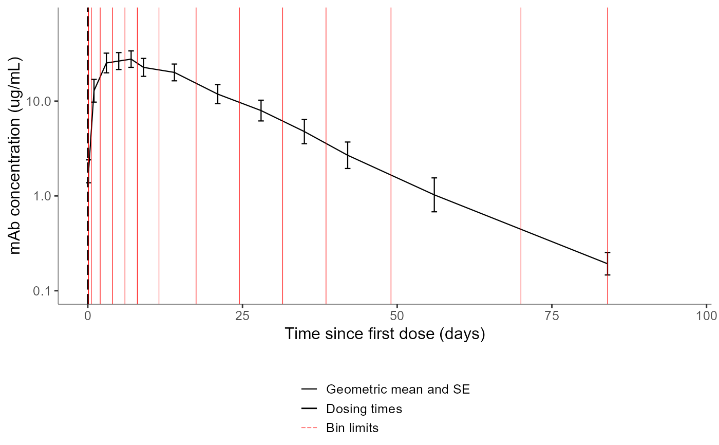
  # changing the settings to display only the mean curve with SE, with bin limits and dosing times
  plotObservedData(settings=list(dots=F,
                            lines=F,
                            mean=T,
                            error=T,
                            meanMethod="geometric",
                            errorMethod="standardError",
                            useCensored=T,
                            binLimits=T,
                            binsSettings=list(criteria="leastsquare", is.fixedNbBins=T, nbBins=20),
                            cens=F,
                            dosingTimes=T,
                            legend=T,
                            grid=F,
                            xlog=F,ylog=T,
                            xlab="Time since first dose (days)",
                            ylab="mAb concentration (ug/mL)",
                            xlim=c(0,96),
                            ylim=c(0.1,70),
                            fontsize=12,
                            units=F))
#> Warning: No shared levels found between `names(values)` of the manual scale and the
#> data's linetype values.
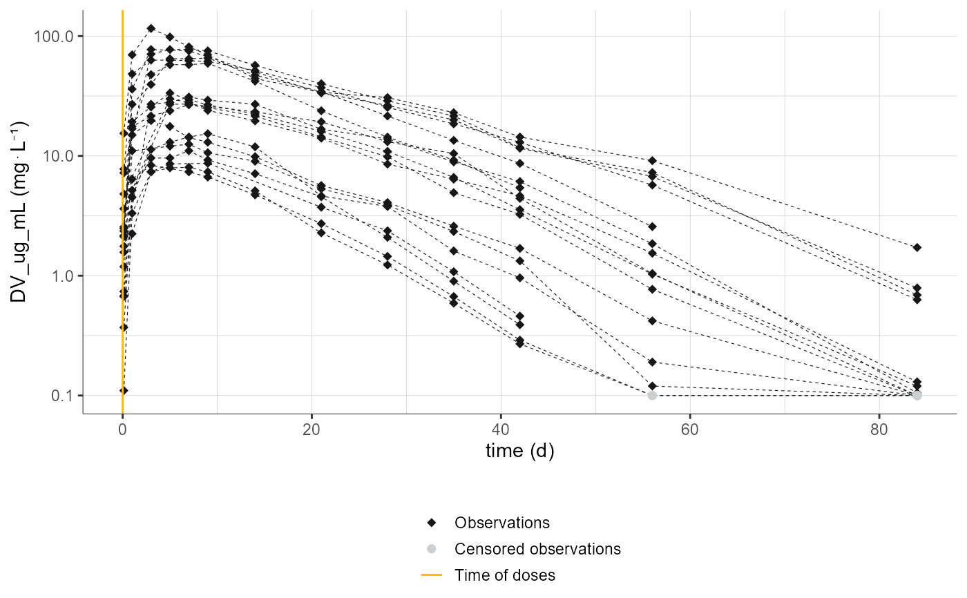
  # changing preferences for observations, censored observations and bin limits
  plotObservedData(settings=list(dots=T, lines=T, legend=T, dosingTimes=T, mean=F, error=F, ylog=T, cens=T),
              preferences=list(obs=list(color="#161617",
                                        radius=2,
                                        shape=18,
                                        lineWidth=0.2,
                                        lineType="dashed",
                                        legend="Observations"),
                               censObs=list(color="#cdced1",
                                            radius=2,
                                            shape=16,
                                            legend="Censored observations"),
                               dosingTimes=list(color="#fcba03",
                                                lineWidth=0.5,
                                                lineType="solid",
                                                legend="Time of doses")))
#> Warning: No shared levels found between `names(values)` of the manual scale and the
#> data's linetype values.
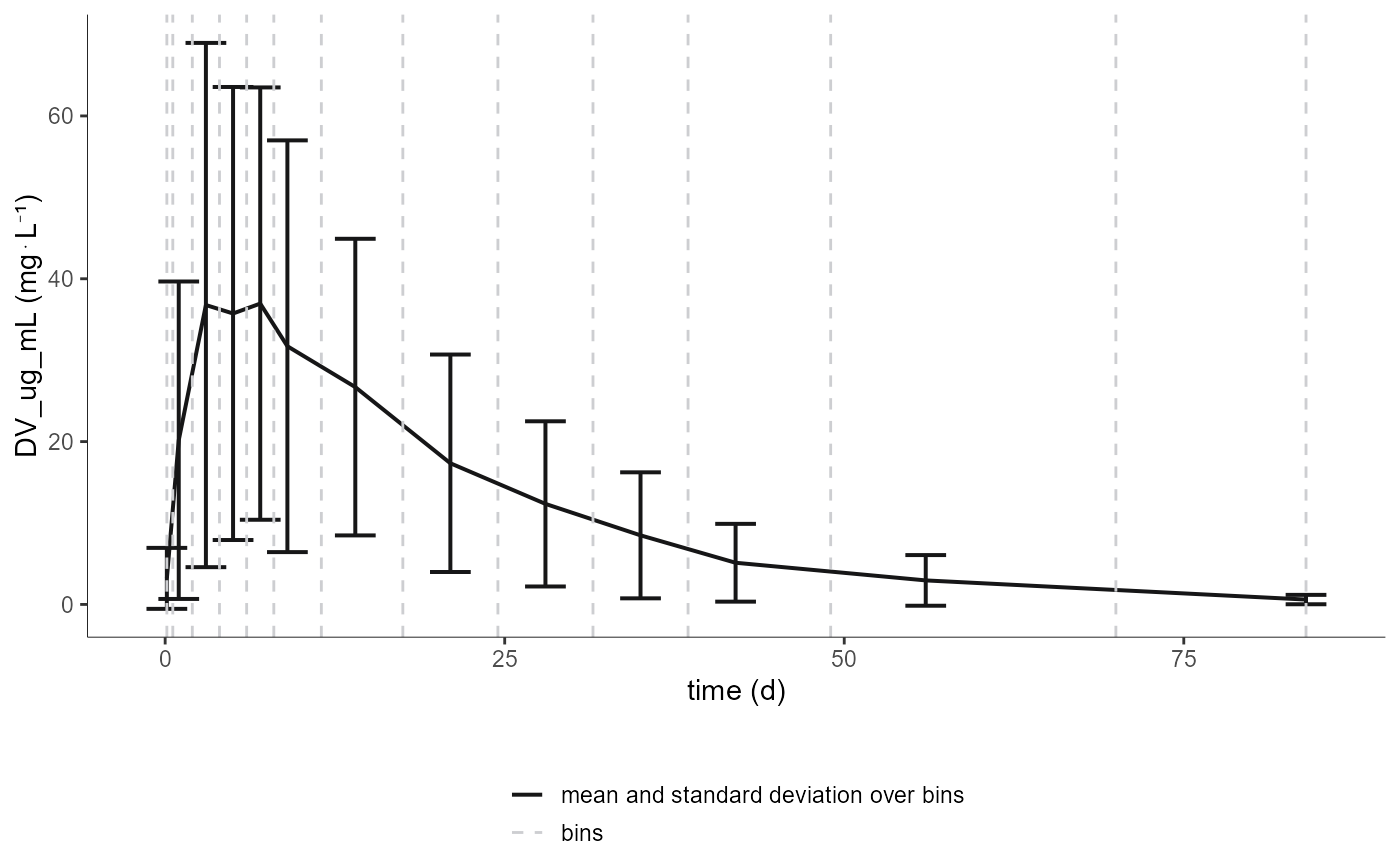
  # changing preferences for mean and bin limits
  plotObservedData(settings=list(dots=F, lines=F, legend=T, binLimits=T, grid=F),
              preferences=list(observationStatistics=list(color="#161617",
                                                          whiskersWidth=3,
                                                          lineWidth=0.7,
                                                          lineType="solid",
                                                          legend="mean and standard deviation over bins"),
                               binsValues=list(color="#cdced1",
                                               lineWidth=0.5,
                                               lineType="dashed",
                                               legend="bins")))
#> Warning: No shared levels found between `names(values)` of the manual scale and the
#> data's linetype values.
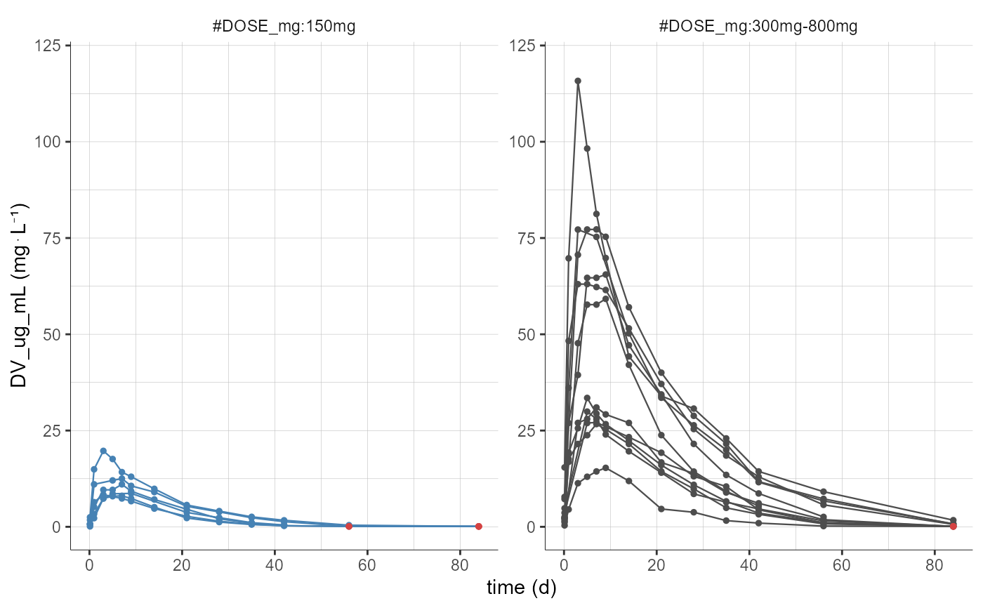
  # color and split by DOSE_mg but grouping two doses levels together
  plotObservedData(settings=list(mean=F,error=F,ylim=c(0,120)),
              stratify = list(groups=list(name="DOSE_mg",definition=list(c("150mg"), c("300mg","800mg"))),
                              color="DOSE_mg",
                              split="DOSE_mg"))
#> Warning: No shared levels found between `names(values)` of the manual scale and the
#> data's linetype values.
  # selecting only one individual
  plotObservedData(settings=list(mean=F,error=F),
                   stratify = list(individualSelection=list(indices=1)))
#> Warning: No shared levels found between `names(values)` of the manual scale and the
#> data's linetype values.
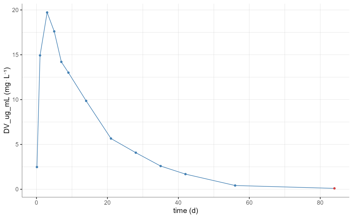
  plotObservedData(settings=list(mean=F,error=F),
                   stratify = list(individualSelection=list(ids="1")))
#> Warning: No shared levels found between `names(values)` of the manual scale and the
#> data's linetype values.

  #============= projects with several covariates to stratify
initializeLixoftConnectors(software = "pkanalix", force=T)
project <- file.path(getDemoPath(), "/2.case_studies/project_Theo_extravasc_SD.pkx")
loadProject(project)

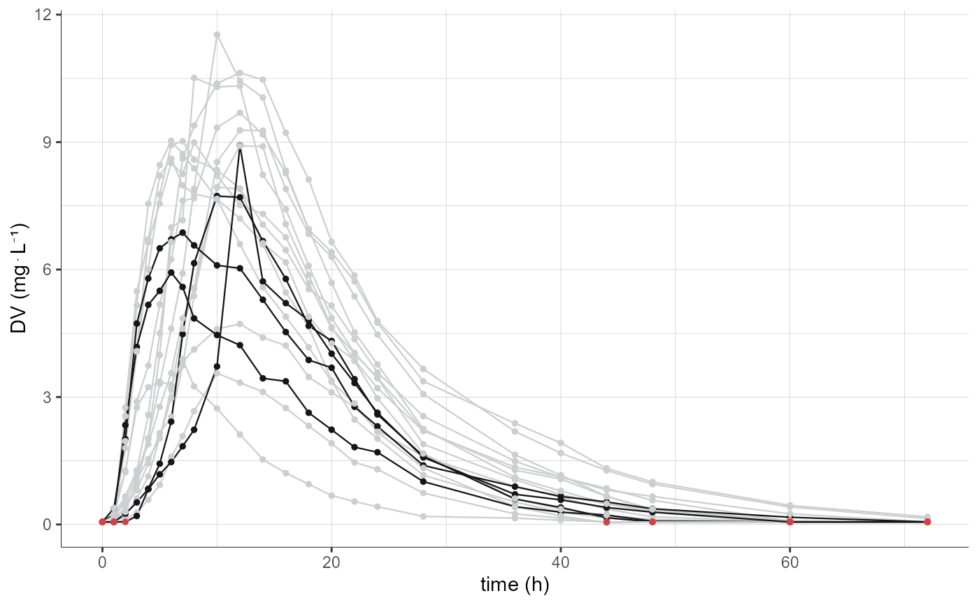
# defining groups for AGE and HT, coloring by HT and filtering by AGE
plotObservedData(settings=list(mean=F,error=F),
            stratify = list(groups=list(list(name="AGE", definition=c(24, 34)),
                                        list(name="HT", definition=c(184.5))),
                            color="HT",
                            colors=c("#cdced1","#161617"),
                            filter=list("AGE",c(1,3))))
#> Warning: No shared levels found between `names(values)` of the manual scale and the
#> data's linetype values.
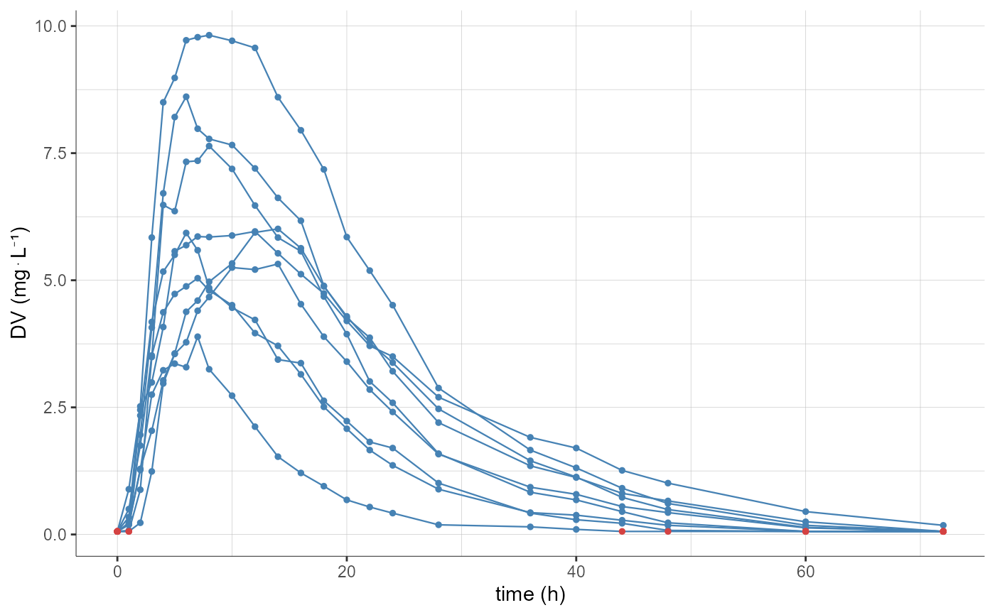
# filter to keep only second sequence (TR) and FORM=test
plotObservedData(settings=list(mean=F,error=F),
            stratify = list(filter=list(list("SEQ",2),list("FORM","test"))))
#> Warning: No shared levels found between `names(values)` of the manual scale and the
#> data's linetype values.
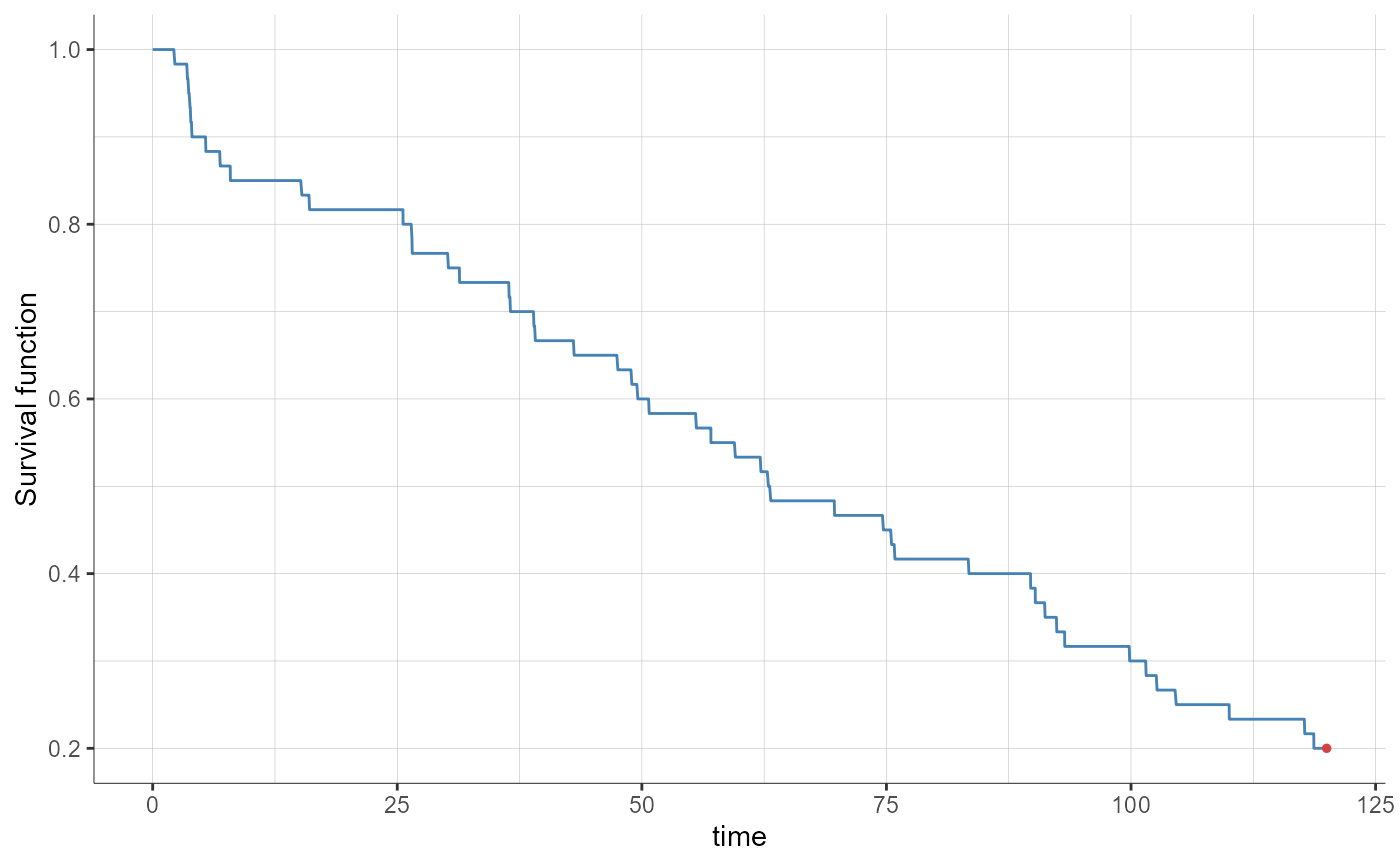
  #============= project with time-to-event data
initializeLixoftConnectors(software = "monolix", force=T)
project <- file.path(getDemoPath(), "/4.joint_models/4.2.continuous_noncontinuous/PKrtte_project.mlxtran")
loadProject(project)

# survival Kaplan-Meier curve
plotObservedData(obsName="Hemorrhaging")
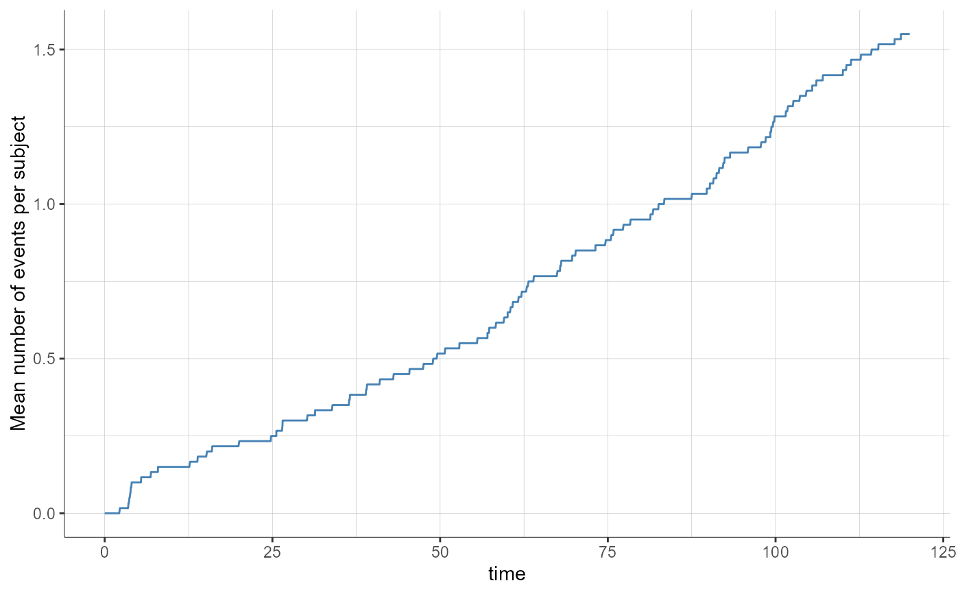
# mean number of events
plotObservedData(obsName="Hemorrhaging",
                 settings=list(eventPlot="averageEventNumber"))
#============= project with categorical data
initializeLixoftConnectors(software = "monolix", force=T)
project <- file.path(getDemoPath(), "/4.joint_models/4.2.continuous_noncontinuous/warfarin_cat_project.mlxtran")
loadProject(project)

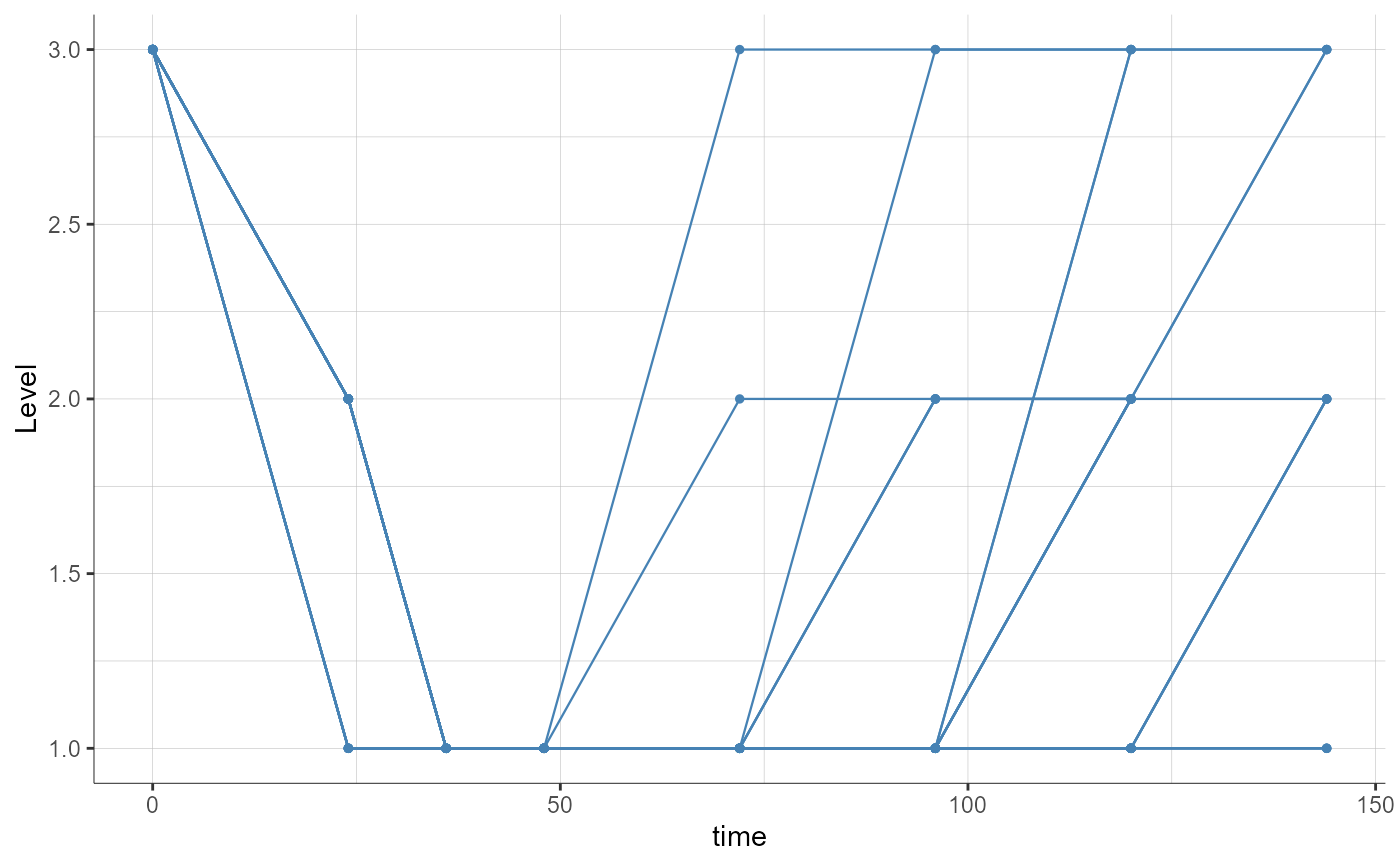
# display is the same as for continuous data by default
plotObservedData(obsName="Level")
#> Warning: No shared levels found between `names(values)` of the manual scale and the
#> data's linetype values.
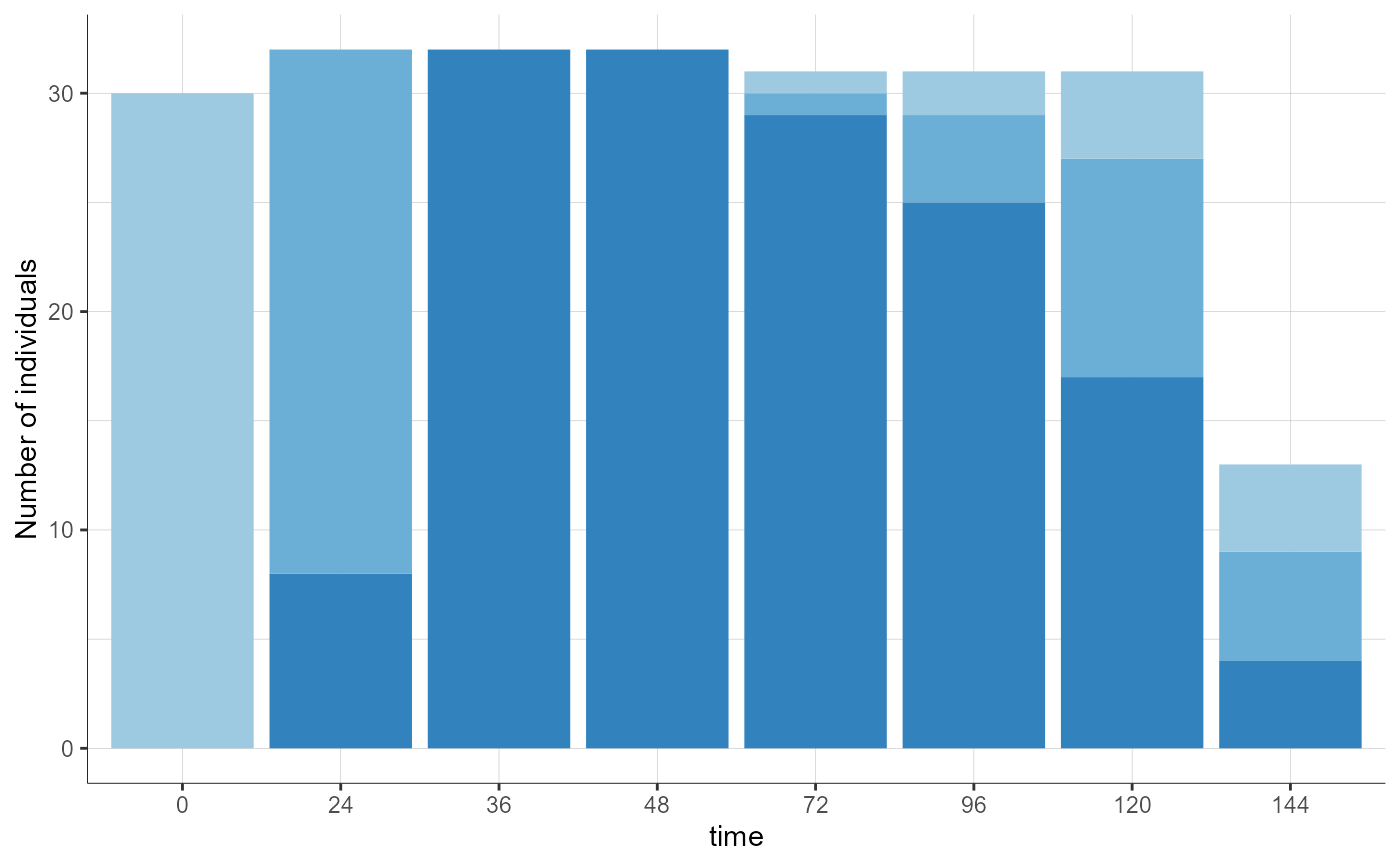
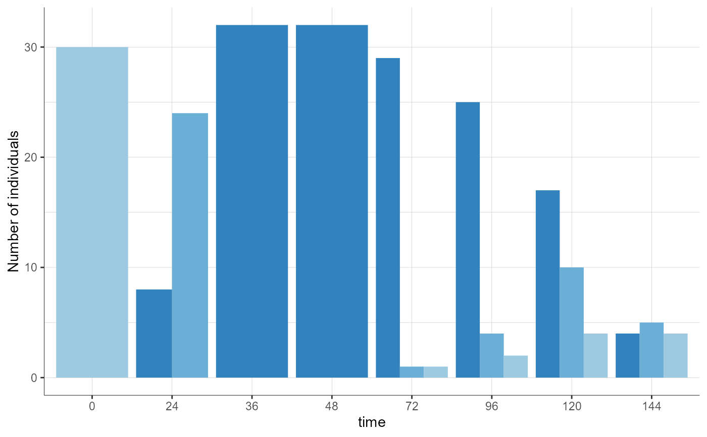
# display as stacked or as grouped
plotObservedData(obsName="Level", settings=list(plot="stacked"))
plotObservedData(obsName="Level", settings=list(plot="grouped"))
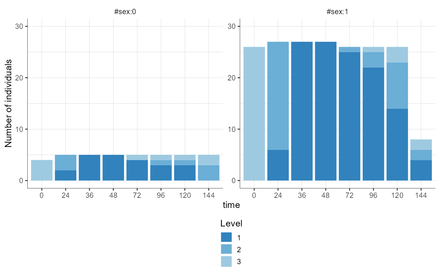
# splitting by sex
plotObservedData(obsName="Level",
                 settings=list(plot="stacked", ylim=c(0,30), legend=T),
                 stratify=list(split="sex"))
#============== project with multiple-dose to show timeAfterLastDose
initializeLixoftConnectors(software = "monolix", force=T)
project <- file.path(getDemoPath(), "/6.PK_models/6.3.multiple_doses/addl_project.mlxtran")
loadProject(project)

# with "time after first dose" by default
plotObservedData()
#> Warning: No shared levels found between `names(values)` of the manual scale and the
#> data's linetype values.

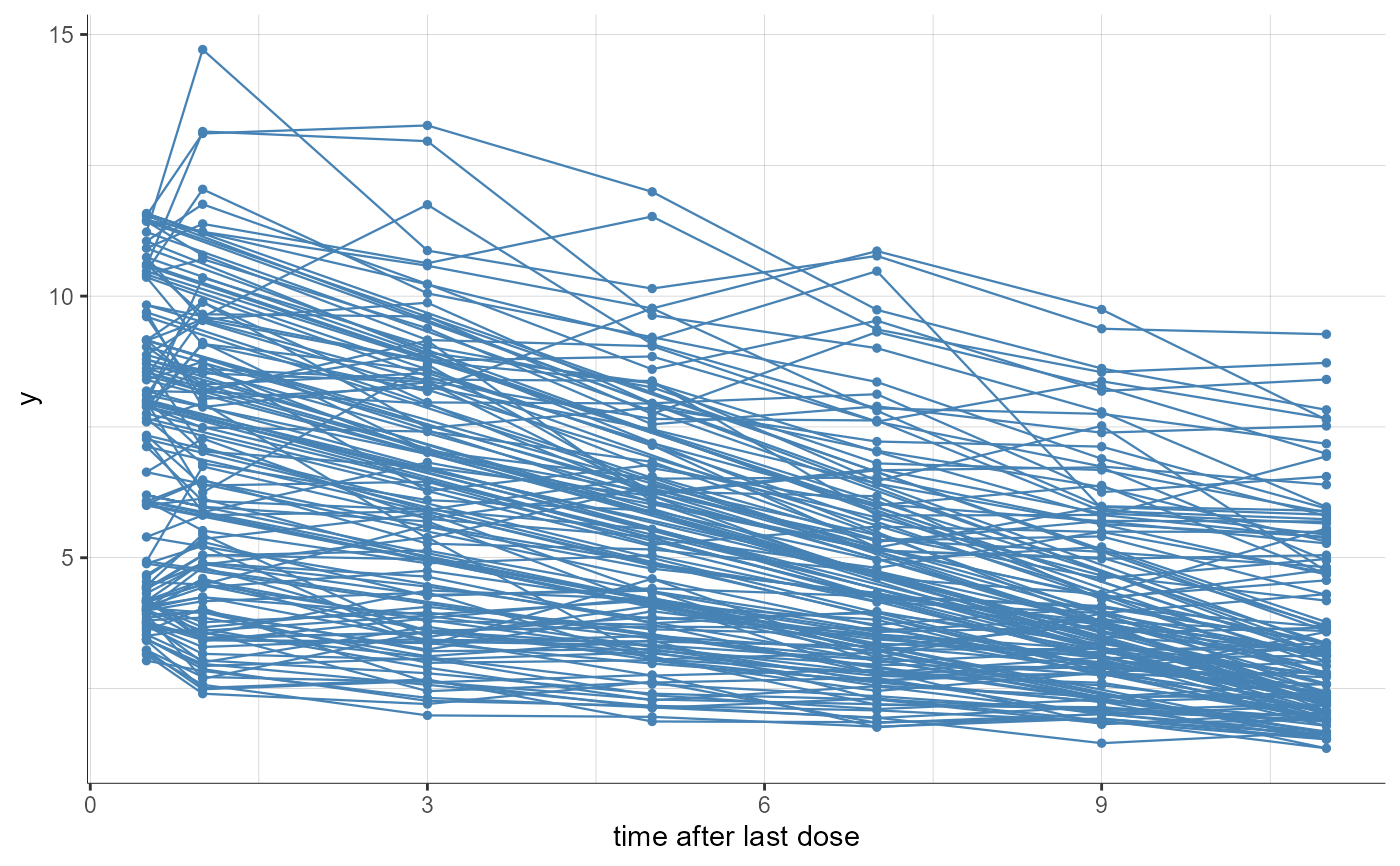
# with "time since previous dose"
plotObservedData(settings=list(timeAfterLastDose=T))
#> Warning: No shared levels found between `names(values)` of the manual scale and the
#> data's linetype values.
#============= project with regressor to show regressor on x-axis
initializeLixoftConnectors(software = "monolix", force=T)
project <- file.path(getDemoPath(), "/7.miscellaneous/7.1.regression_variables/reg3_warfarinPD_linearInterp_project.mlxtran")
loadProject(project)
#> [ERROR] Cannot load the project from its file 'C:/Users/FranoMihaljevic/lixoft/monolix/monolix2024R1/demos/7.miscellaneous/7.1.regression_variables/reg3_warfarinPD_linearInterp_project.mlxtran', as this file could not be found.

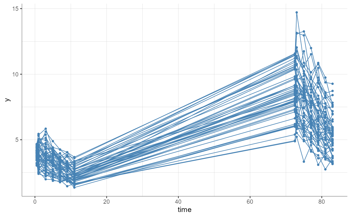
# with "time" on x-axis by default
plotObservedData()
#> Warning: No shared levels found between `names(values)` of the manual scale and the
#> data's linetype values.
# with regressor "Cc" (concentration) on x-axis
plotObservedData(settings=list(xvariable="Cc"))
#> Error: Invalid setting 'xvariable': no regressor called 'Cc' in the dataset

#============= project with nominal time on x-axis
initializeLixoftConnectors(software = "pkanalix", force=T)
project <- file.path(getDemoPath(), "/1.basic_examples/project_nominal_time.pkx")
loadProject(project)

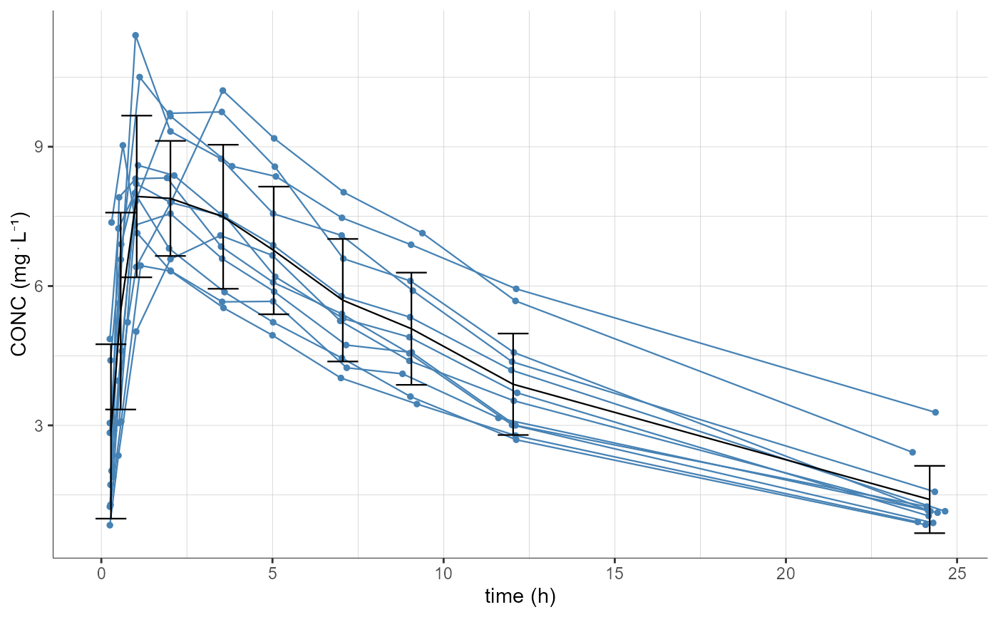
# with "actual time" by default
plotObservedData()
#> Warning: No shared levels found between `names(values)` of the manual scale and the
#> data's linetype values.
# with nominal time on x-axis
plotObservedData(settings=list(xvariable="nominalTime"))
#> Warning: No shared levels found between `names(values)` of the manual scale and the
#> data's linetype values.
