
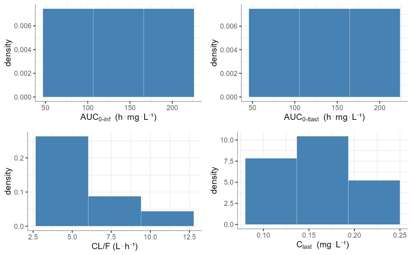
[PKanalix] Distribution of the individual NCA parameters
Plot the distribution of the individual NCA parameters.
Usage
plotNCAParametersDistribution(
  parameters = NULL,
  settings = list(),
  preferences = list(),
  stratify = list()
)
Arguments
parameters (vector) vector of NCA parameters to display. (by default the first 12 computed NCA parameters are displayed). settings List with the following settings:plot (character) Type of plot: probability density distribution as histogram ("pdf", default), or cumulative density distribution ("cdf"). legend (logical) If TRUE, plot legend is displayed (default FALSE). grid (logical) If TRUE, plot grid is displayed (default TRUE). ncol (integer) number of columns to arrange subplots (default 4). fontsize (integer) Font size of text elements (default 11). units (logical) If TRUE, units are added in axis labels (default TRUE). scales (character) Should scales be fixed ("fixed"), free ("free", default), or free in one dimension ("free_x", "free_y"). preferences (optional) preferences for plot display, run getPlotPreferences("plotNCAParametersDistribution") to check available options. stratify List with the stratification arguments:groups - Definition of stratification groups. By default, stratification groups are already defined as one group for each category for categorical covariates, and two groups of equal number of individuals for continuous covariates. To redefine groups, for each covariate to redefine, specify a list with:namecharactercovariate name (e.g "AGE")definitionvector(continuous) || list>(categorical)For continuous covariates, vector of break values (e.g c(35, 65)). For categorical covariates, groups of categories as a list of vectors(e.g list(c("study101"), c("study201","study202"))) split (vector) - Vector of covariates used to split (i.e facet) the plot (by default no split is applied). For instance c("FORM","AGE"). filter (list< list> >) - List of pairs containing a covariate name and the vector of indexes or categories (for categorical covariates) of the groups to keep (by default no filtering is applied). For instance, list("AGE",c(1,3)) to keep the individuals belonging to the first and third age group, according to the definition in groups. For instance, list("FORM","ref") using the category name for categorical covariates.
Value
-
A ggplot object if only one parameter is specified in
parameters -
A TableGrob object if multiple plots (output of grid.arrange)
See also
getChartsData getPlotPreferences
Examples
initializeLixoftConnectors(software = "pkanalix")
project <- file.path(getDemoPath(), "/2.case_studies/project_Theo_extravasc_SD.pkx")
loadProject(project)
runNCAEstimation()
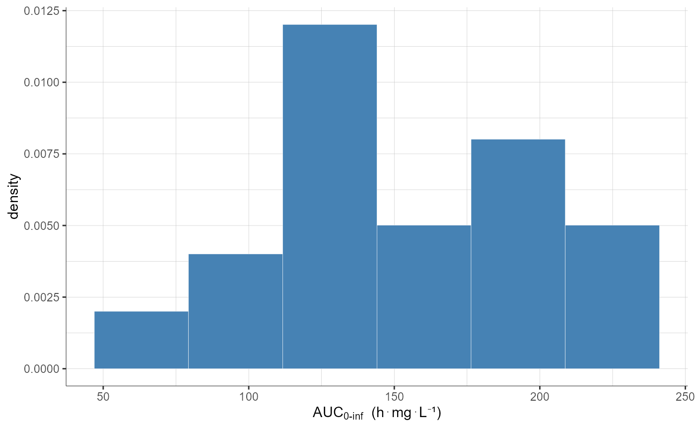
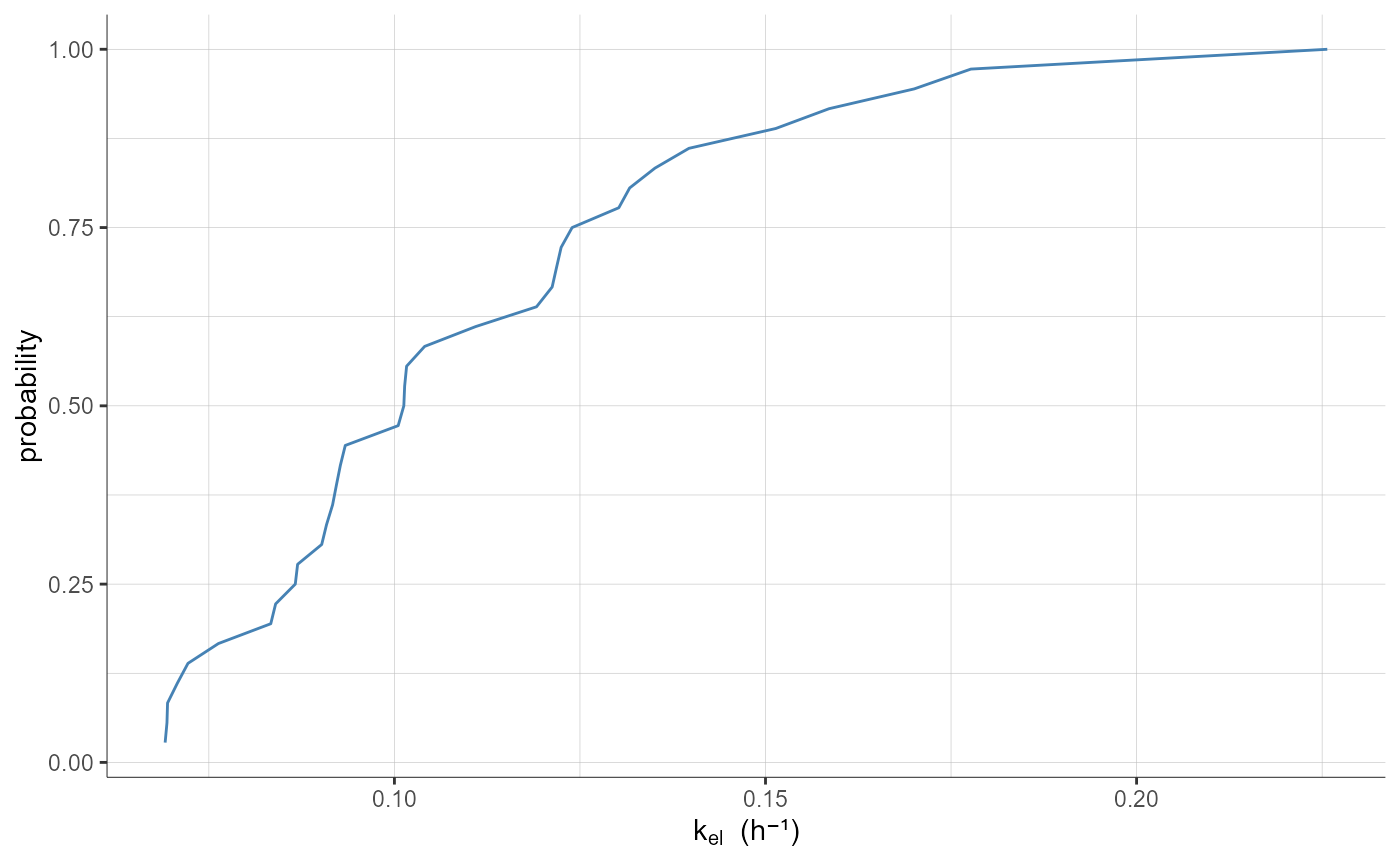
# plot a single parameter, as pdf or cdf
plotNCAParametersDistribution(parameters = "AUCINF_obs", settings = list(plot = "pdf"))
plotNCAParametersDistribution(parameters = "Lambda_z", settings = list(plot = "cdf"))
# with a single parameter, a ggplot object if returned and additional ggplot elements can be added
library(ggplot2)
plotNCAParametersDistribution(parameters = "AUCINF_obs")+geom_vline(xintercept=140)

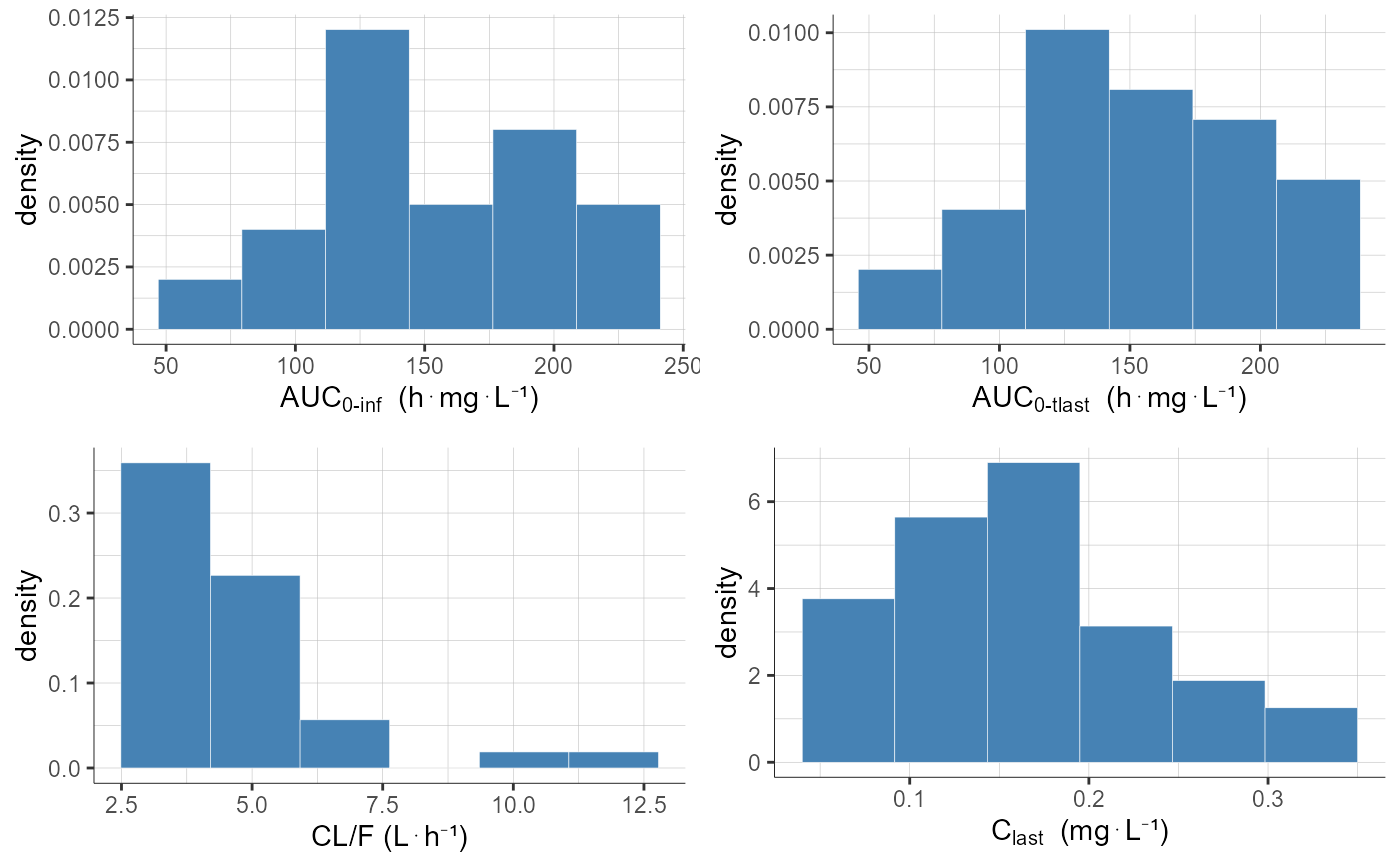
# display only 4 parameters in a 2x2 matrix (ncol=2)
plotNCAParametersDistribution(parameters = c('AUCINF_obs', 'AUClast', 'Cl_F_obs', 'Clast'),
                              settings = list(ncol=2))
#> TableGrob (1 x 1) "arrange": 1 grobs
#> z cells name grob
#> 1 1 (1-1,1-1) arrange gtable[arrange]
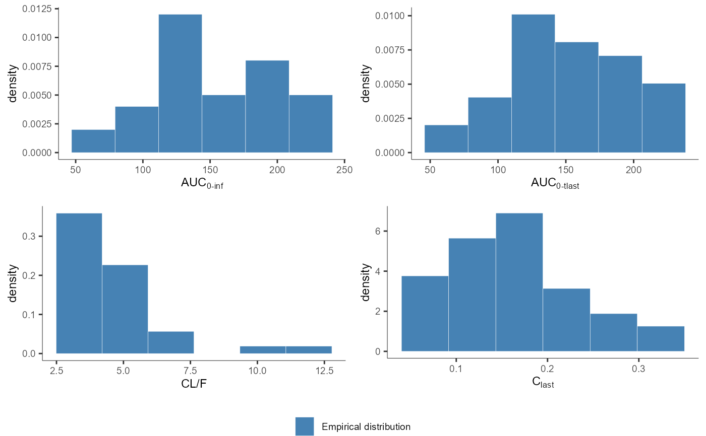
# changing the settings to choose which elements to display
plotNCAParametersDistribution(parameters = c('AUCINF_obs', 'AUClast', 'Cl_F_obs', 'Clast'),
settings = list(ncol=2,
units=F,
legend=T,
grid=F,
fontsize=9))
#> TableGrob (2 x 1) "arrange": 2 grobs
#> z cells name grob
#> 1 1 (1-1,1-1) arrange gtable[arrange]
#> 2 2 (2-2,1-1) arrange gtable[guide-box]
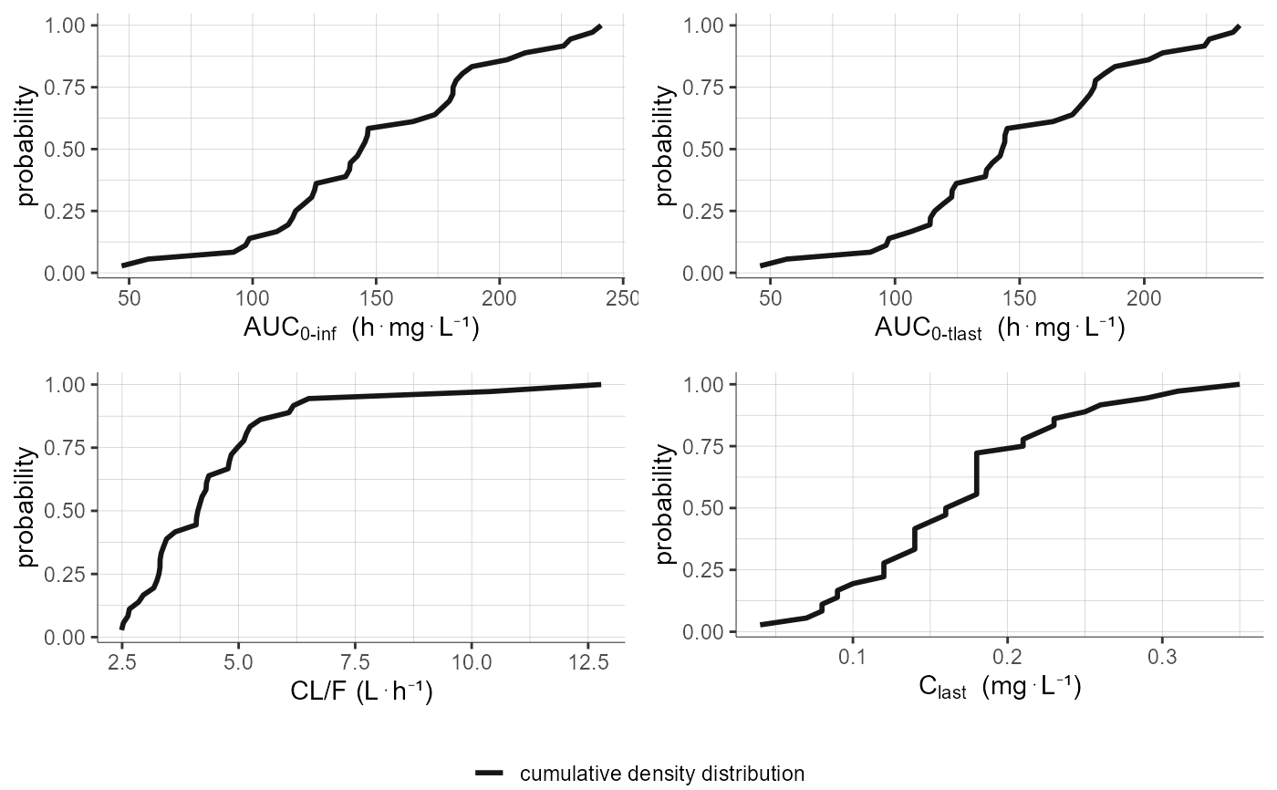
# changing the preferences (appearance of the elements) when using plot="cdf"
plotNCAParametersDistribution(parameters = c('AUCINF_obs', 'AUClast', 'Cl_F_obs', 'Clast'),
settings = list(ncol=2, legend=T, plot="cdf"),
preferences = list(empirical=list(color="#161617",
lineWidth=1,
lineType="solid",
legend="cumulative density distribution")))
#> TableGrob (2 x 1) "arrange": 2 grobs
#> z cells name grob
#> 1 1 (1-1,1-1) arrange gtable[arrange]
#> 2 2 (2-2,1-1) arrange gtable[guide-box]
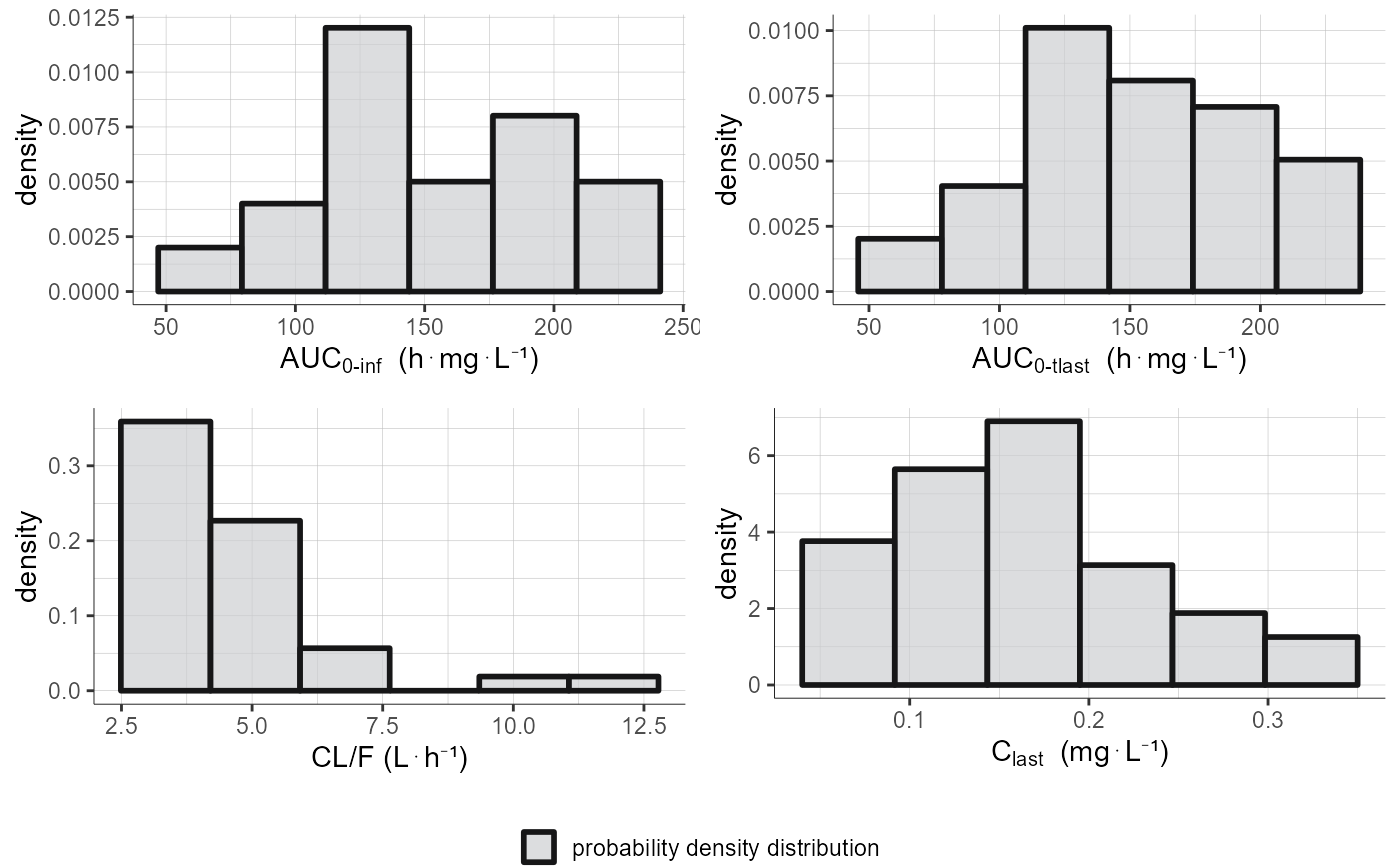
# changing the preferences (appearance of the elements) when using plot="pdf"
plotNCAParametersDistribution(parameters = c('AUCINF_obs', 'AUClast', 'Cl_F_obs', 'Clast'),
settings = list(ncol=2, legend=T, plot="pdf"),
preferences = list(histogramBar=list(fill="#cdced1",
opacity=0.7,
stroke="#161617",
strokeWidth=1,
legend="probability density distribution")))
#> TableGrob (2 x 1) "arrange": 2 grobs
#> z cells name grob
#> 1 1 (1-1,1-1) arrange gtable[arrange]
#> 2 2 (2-2,1-1) arrange gtable[guide-box]
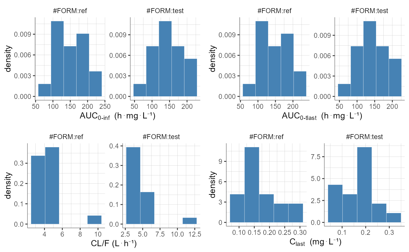
# split each plot into two subplots for FORM=ref and FORM=test
plotNCAParametersDistribution(parameters = c('AUCINF_obs', 'AUClast', 'Cl_F_obs', 'Clast'),
settings = list(ncol=2),
stratify = list(split=c("FORM")))
#> TableGrob (1 x 1) "arrange": 1 grobs
#> z cells name grob
#> 1 1 (1-1,1-1) arrange gtable[arrange]
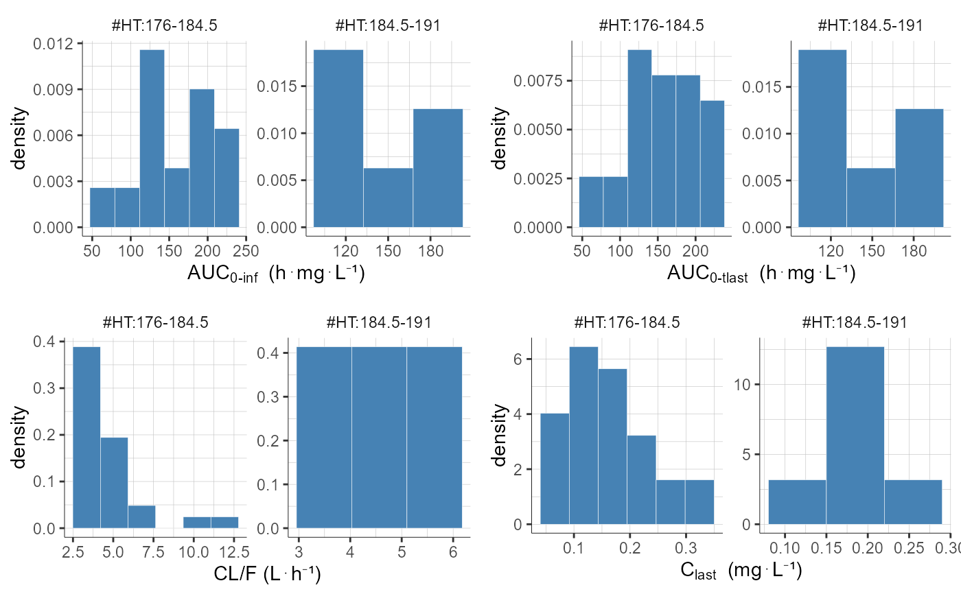
# define groups for AGE and HT, filter by AGE and split by HT
plotNCAParametersDistribution(parameters = c('AUCINF_obs', 'AUClast', 'Cl_F_obs', 'Clast'),
settings=list(ncol=2),
stratify = list(groups=list(list(name="AGE", definition=c(30, 35)),
list(name="HT", definition=c(184.5))),
filter=list("AGE",c(1,3)),
split="HT"))
#> TableGrob (1 x 1) "arrange": 1 grobs
#>   z     cells    name            grob
#> 1 1 (1-1,1-1) arrange gtable[arrange]

# filter to keep only second sequence (TR) and Period=1
plotNCAParametersDistribution(parameters = c('AUCINF_obs', 'AUClast', 'Cl_F_obs', 'Clast'),
                              settings=list(ncol=2),
                              stratify = list(filter=list(list("SEQ",2),list("Period","1"))))
#> TableGrob (1 x 1) "arrange": 1 grobs
#>   z     cells    name            grob
#> 1 1 (1-1,1-1) arrange gtable[arrange]