plotCovariates

Plot the covariates.

Usage

        R
    
plotCovariates(
  covariatesRows = NULL,
  covariatesColumns = NULL,
  settings = list(),
  preferences = list(),
  stratify = list()
)

Arguments

covariatesRows

vector with the name of covariates to display on rows (by default the first 4 covariates are displayed).

covariatesColumns

vector with the name of covariates to display on columns (by default the first 4 covariates are displayed).

settings

List with the following settings

regressionLine (logical) If TRUE, Add regression line in scatterplots (default TRUE).
spline (logical) If TRUE, Add xpline in scatterplots (default FALSE).
histogramColors (vector) List of colors to use in histograms plots.
histogramPosition (character) Type of histogram: "stacked", "grouped" or "default" (histograms with categorical covariates in xaxis the plot is grouped else it is stacked), (Default is "default")
legend (logical) add (TRUE) / remove (FALSE) plot legend (default FALSE).
grid (logical) add (TRUE) / remove (FALSE) plot grid (default TRUE).
ncol (integer) number of columns when facet = TRUE (default 4).
bins (integer) number of bins for the histogram (default 10)
fontsize (integer) Plot text font size.

preferences

(optional) preferences for plot display, run getPlotPreferences("plotCovariates") to check available displays.

stratify

List with the stratification arguments:

groups - Definition of stratification groups. By default, stratification groups are already defined as one group for each category for categorical covariates, and two groups of equal number of individuals for continuous covariates. To redefine groups, for each covariate to redefine, specify a list with:

name	character	covariate name (e.g `"AGE"`)
definition	(vector(continuous) \|\| list>(categorical))	For continuous covariates, vector of break values (e.g `c(35, 65)`). For categorical covariates, groups of categories as a list of vectors(e.g `list(c("study101"), c("study201","study202"))`)

split (vector) - Vector of covariates used to split (i.e facet) the plot (by default no split is applied). For instance c("FORM","AGE").
filter (list< list> >) - List of pairs containing a covariate name and the vector of indexes or categories (for categorical covariates) of the groups to keep (by default no filtering is applied). For instance, list("AGE",c(1,3)) to keep the individuals belonging to the first and third age group, according to the definition in groups. For instance, list("FORM","ref") using the category name for categorical covariates.
color (vector) - Vector of covariates used for coloring (by default no coloring is applied). For instance c("FORM","AGE").
colors - Vector of colors to use when color argument is used. Takes precedence over colors defined in preferences. For instance c("#ebecf0","#cdced1","#97989c").
individualSelection - Ids to display (by default the 12 first ids are displayed) defined as:
- indices (vector) - Indices of the individuals to display (by default, the 12 first individuals are selected). If occasions are present, all occasions of the selected individuals will be displayed. Takes precedence over ids. For instance c(5,6,10,11).
- isRange (logical) - If TRUE, all individuals whose index is inside [min(indices), max[indices]] are selected (FALSE by default). Forced to FALSE if ids is defined.
- ids (vector) - Names of the individuals to display. If occasions are present, all occasions of the selected individuals will be displayed. For instance c("101-01","101-02","101-03"). If ids are integers, can also be c(1,3,6). Ignored if indices is defined.

Value

A ggplot object if one element in covariatesRows and covariatesColumns,
A TableGrob object if multiple plots (output of grid.arrange)

Details

Generate scatterplots between two continuous covariates or bar plot between categorical covariates.

Examples

R

  initializeLixoftConnectors(software = "pkanalix")
  project <- file.path(getDemoPath(), "2.case_studies/project_Theo_extravasc_SD.pkx")
  loadProject(project)

  # covariate distribution when only one covariate is specified
  plotCovariates(covariatesRows = "HT", settings = list(bins = 10))

R


#> TableGrob (1 x 1) "arrange": 1 grobs
#>   z     cells    name            grob
#> 1 1 (1-1,1-1) arrange gtable[arrange]

  # scatter plot when both covariates are continuous
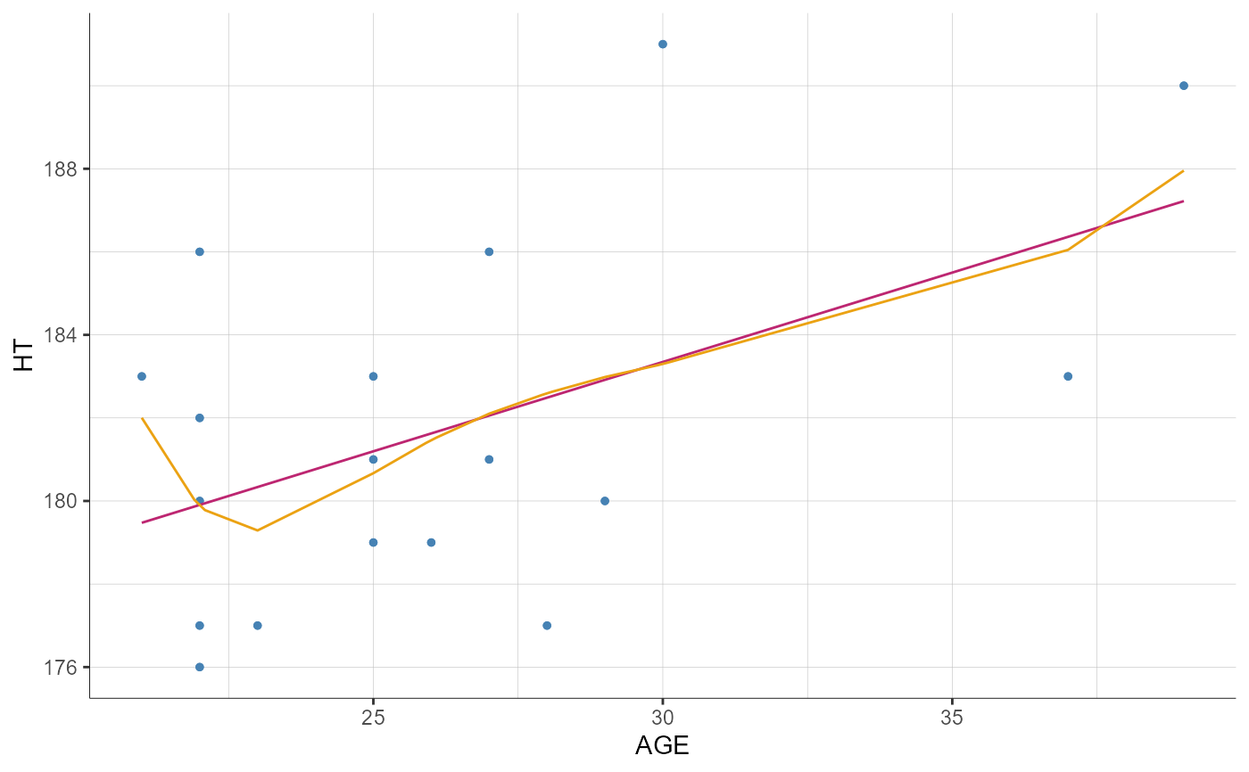
  plotCovariates(covariatesRows = "HT", covariatesColumns = "AGE", settings = list(spline = TRUE))

R


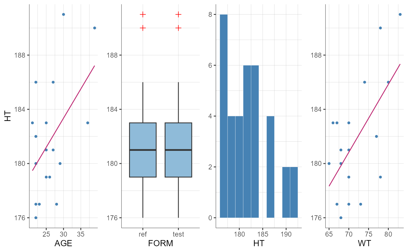
  plotCovariates(covariatesRows = "HT", covariatesColumns = c("AGE", "FORM"))

R


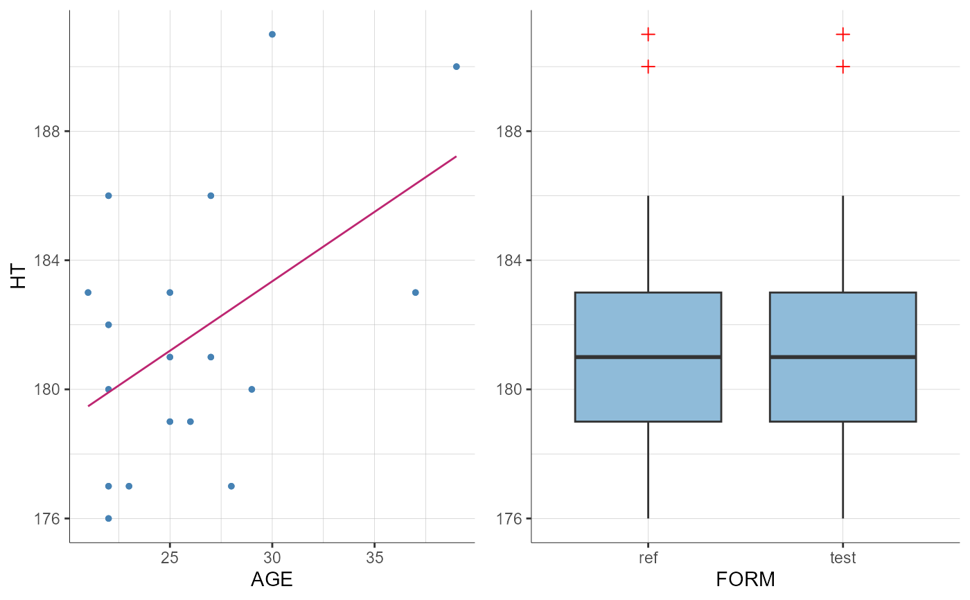
#> TableGrob (1 x 1) "arrange": 1 grobs
#>   z     cells    name            grob
#> 1 1 (1-1,1-1) arrange gtable[arrange]

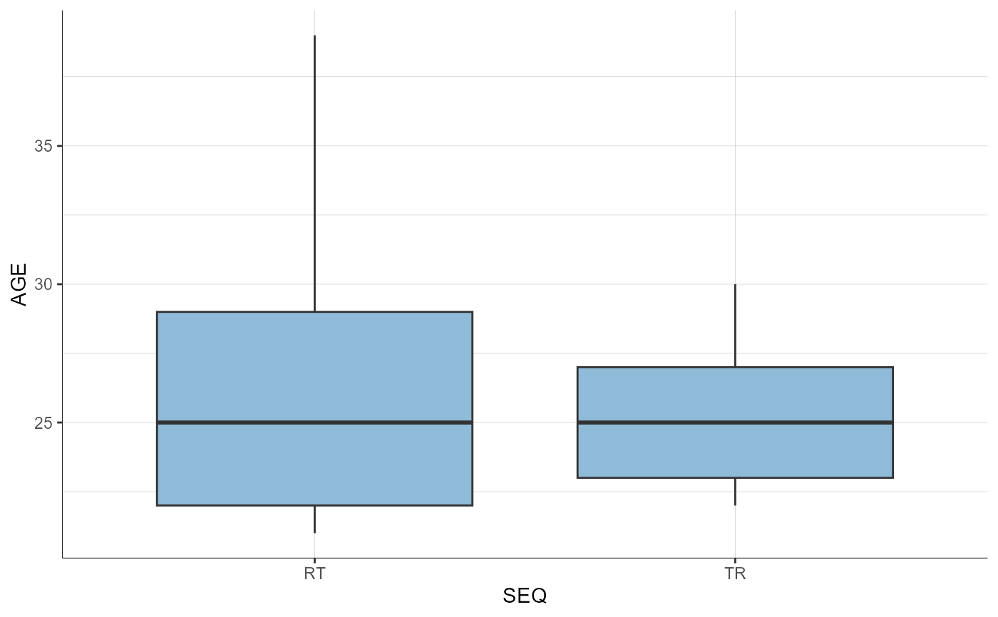
  # box plot when one covariate is categorical and the othe one is continuous
  preferences <- list(boxplot = list(fill = "#2075AE"), boxplotOutlier = list(shape = 3))
  plotCovariates(covariatesRows = "FORM", covariatesColumns = "AGE", preferences = preferences)

R



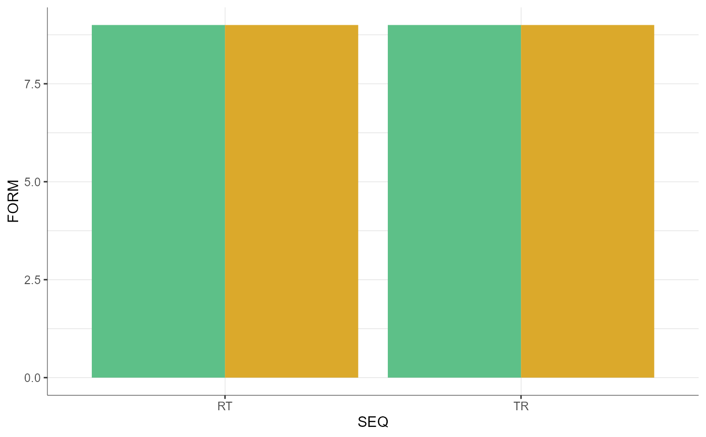
  # histogram when covariate on column is categorical
  plotCovariates(covariatesRows = "FORM", covariatesColumns = "SEQ",
                 settings = list(histogramColors = c("#5DC088", "#DBA92B")))

R


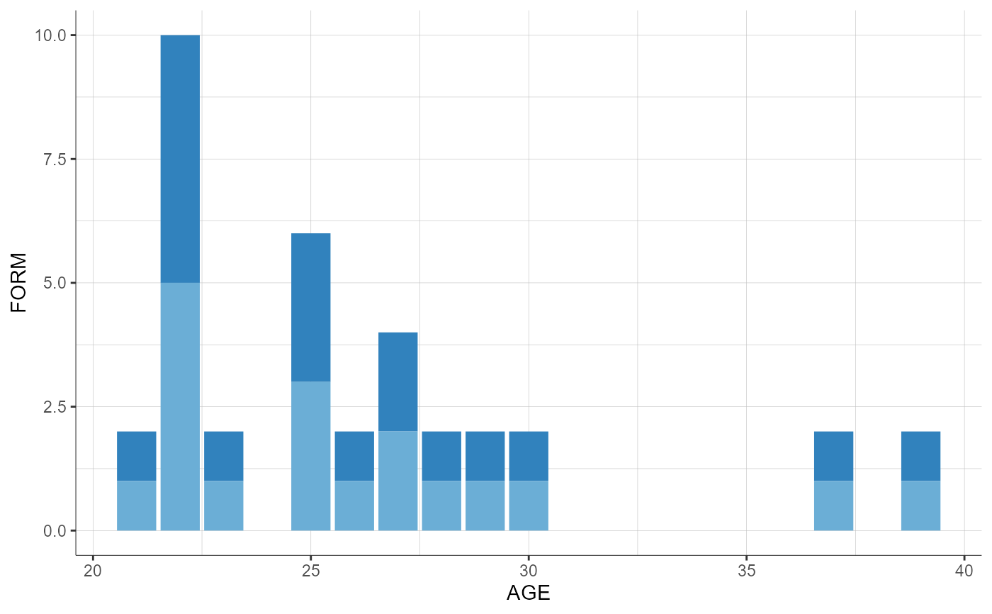
  plotCovariates(covariatesRows = "AGE", covariatesColumns = "SEQ",
                 settings = list(histogramColors = c("#5DC088", "#DBA92B")))

R



  # stratification
  plotCovariates(covariatesRows = "HT", covariatesColumns = "WT",
                 stratify = list(split = "AGE",
                                 filter = list("Period", 1),
                                 groups = list(name = "AGE", definition = 25)))

R


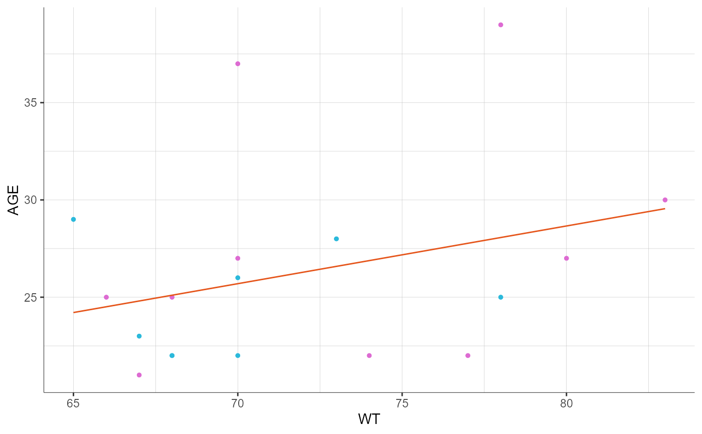
  preferences <- list(regressionLine = list(color = "#E5551B"))
  plotCovariates(covariatesRows = "AGE", covariatesColumns = "WT",
                 stratify = list(color = "HT",
                                 groups = list(name = "HT", definition = 181),
                                 colors = c("#2BB9DB", "#DD6BD2")),
                 preferences = preferences)

R


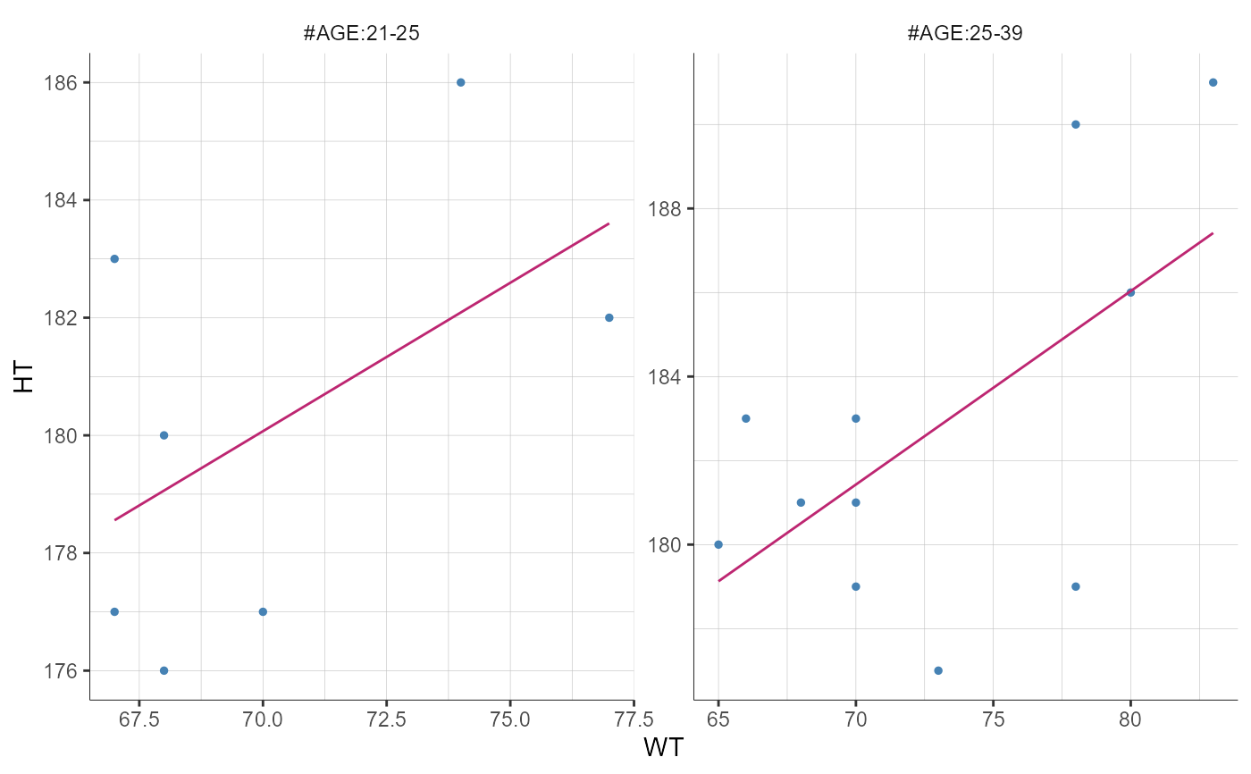
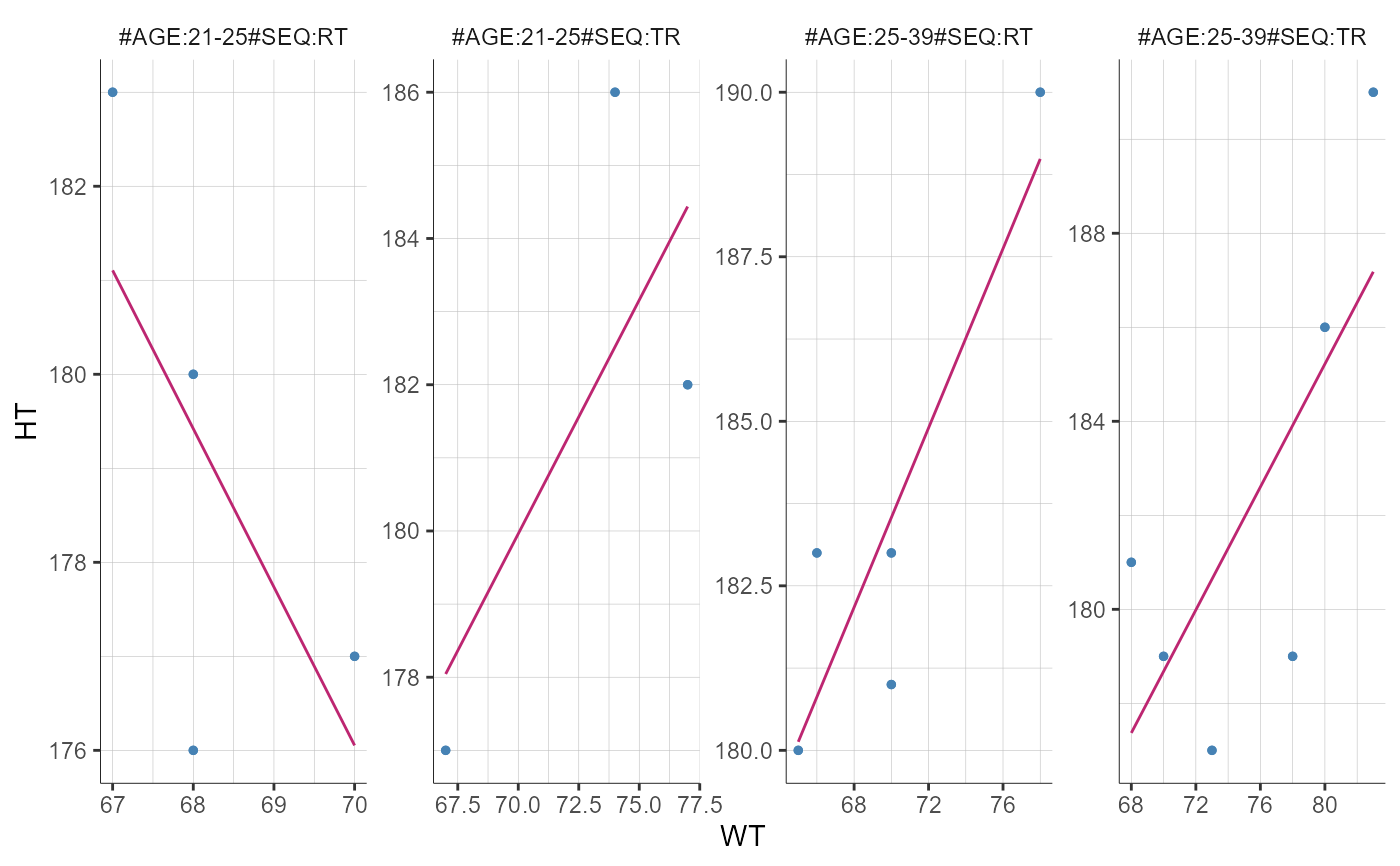
  plotCovariates(covariatesRows = "HT", covariatesColumns = "WT",
                 stratify = list(split = c("AGE", "SEQ"),
                                 groups = list(name = "AGE", definition = 25)))

R



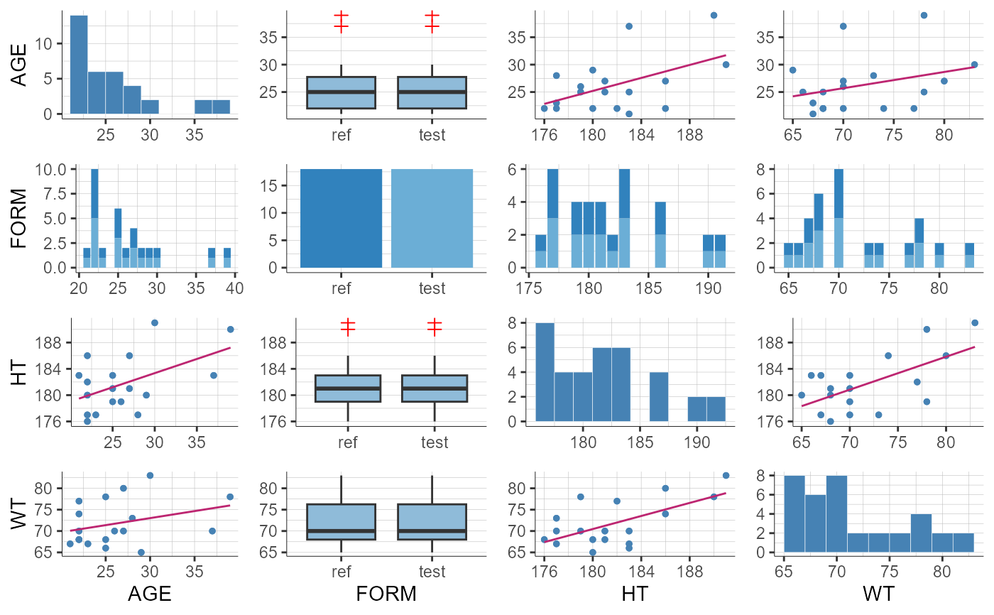
  # Mulitple covariates
  plotCovariates()

R


#> TableGrob (1 x 1) "arrange": 1 grobs
#>   z     cells    name            grob
#> 1 1 (1-1,1-1) arrange gtable[arrange]
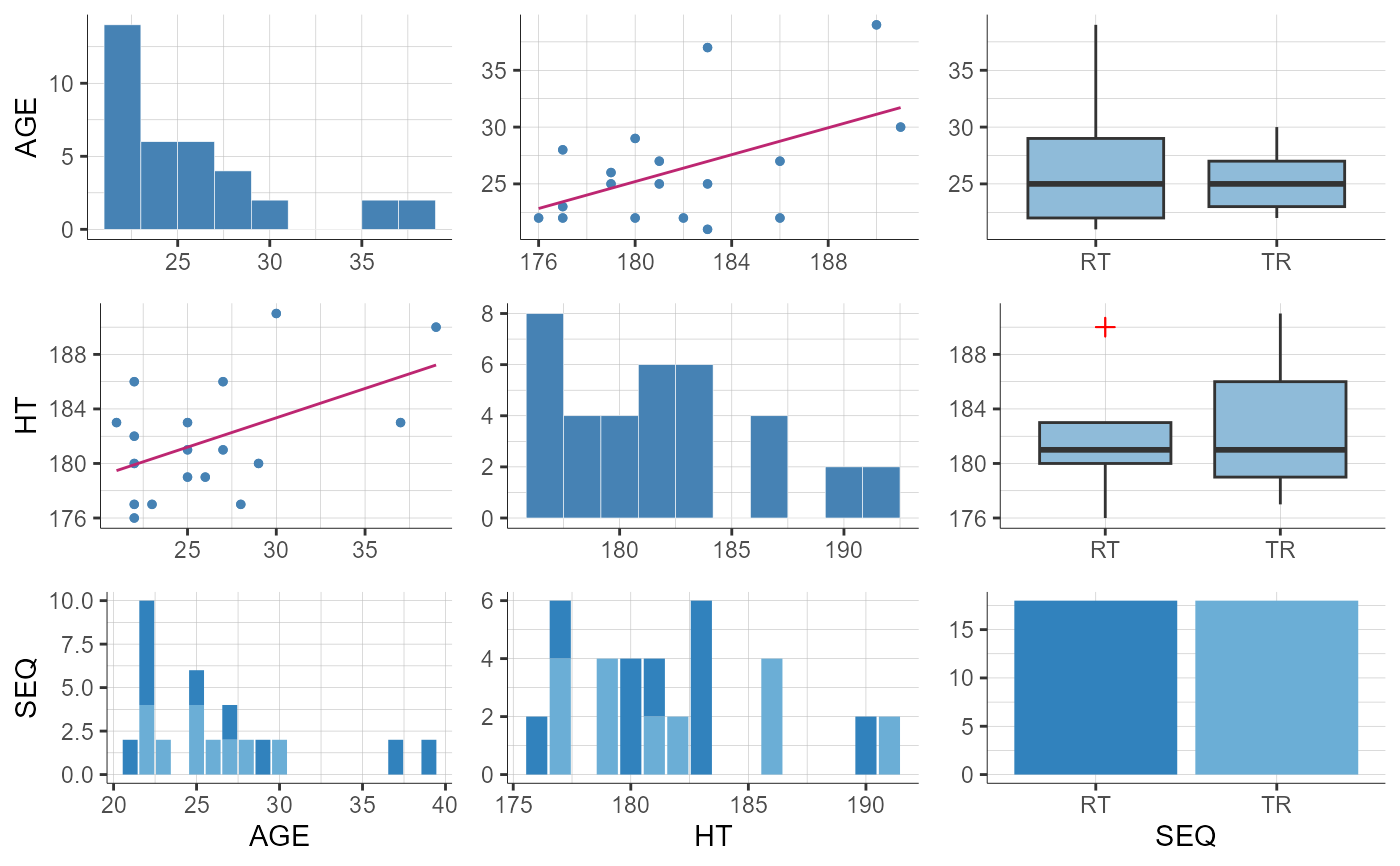
  plotCovariates(covariatesRows = c("AGE", "SEQ", "HT"), covariatesColumns = c("AGE", "SEQ", "HT"))

R


#> TableGrob (1 x 1) "arrange": 1 grobs
#>   z     cells    name            grob
#> 1 1 (1-1,1-1) arrange gtable[arrange]
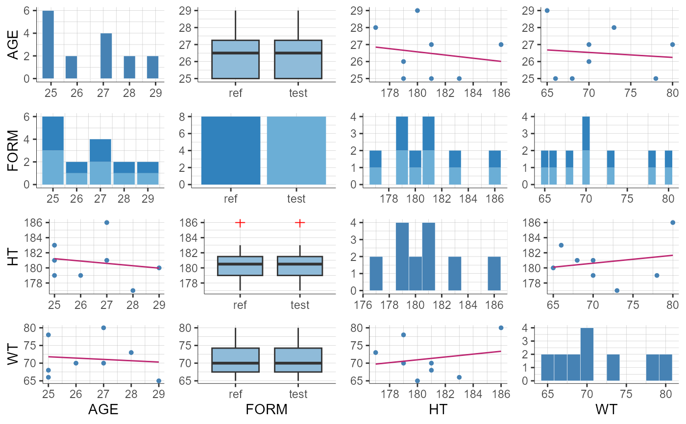
  plotCovariates(stratify = list(filter = list("AGE", 2),
                                 groups = list(name = "AGE", definition = c(25, 30))))

R


#> TableGrob (1 x 1) "arrange": 1 grobs
#>   z     cells    name            grob
#> 1 1 (1-1,1-1) arrange gtable[arrange]