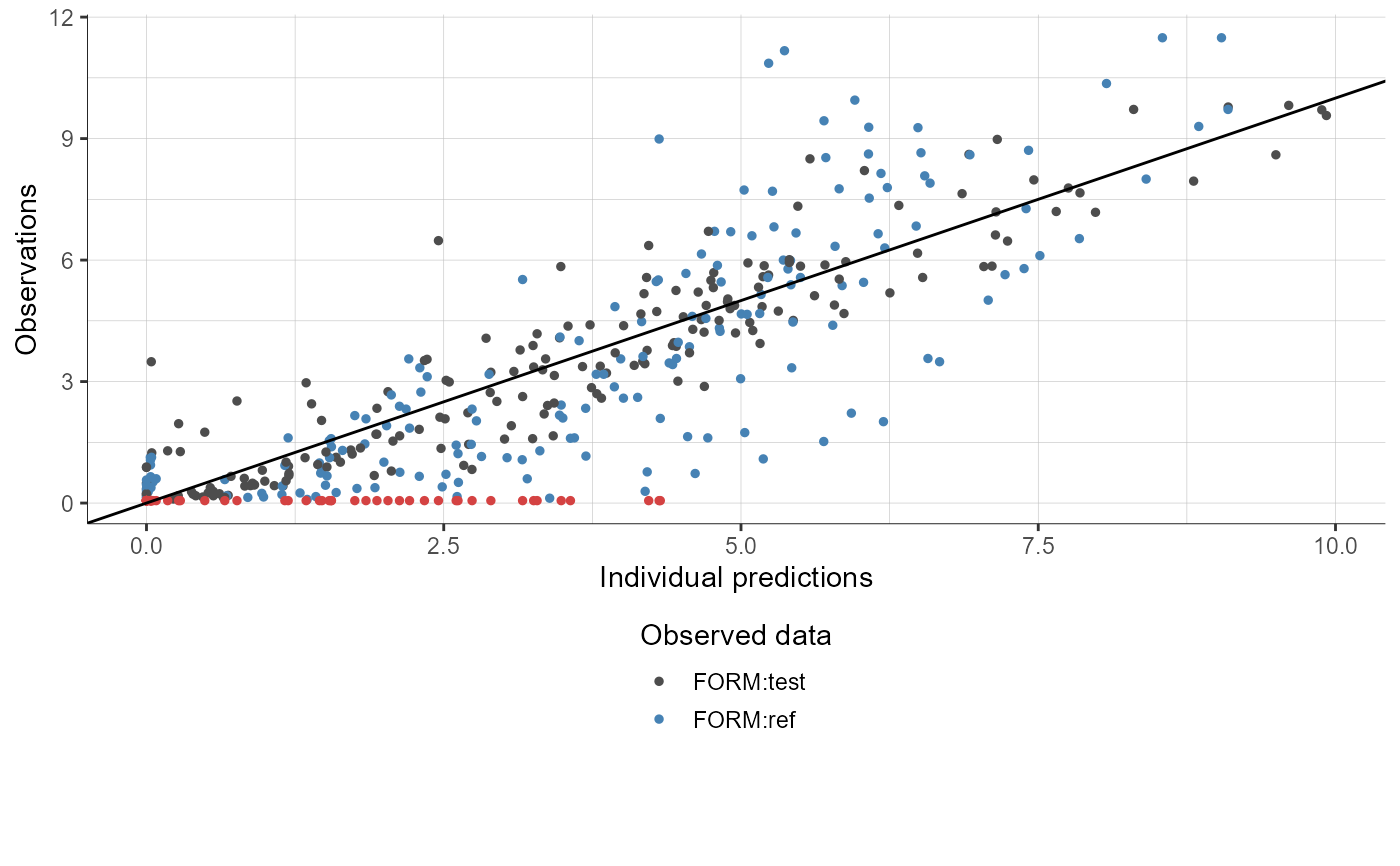
[PKanalix] Plot observations vs the CA predictions.
Plot the observations vs the CA predictions.
Usage
plotCAObservationsVsPredictions(
  obsName = NULL,
  settings = list(),
  preferences = list(),
  stratify = list()
)
Arguments
obsName (character) Name of the observation (if several OBS ID are used). By default the first observation id is considered. settings List with the following settings:useCensored (logical) Choose to use BLQ data (TRUE) or to ignore it (FALSE, default) to compute the spline. obs (logical) - If TRUE, observations are displayed as dots (default TRUE). cens (logical) - If TRUE, censored observations are displayed as red dots (default TRUE). spline (logical) - If TRUE, spline is displayed (default FALSE). identityLine (logical) - If TRUE, identity line y=x is displayed (default TRUE). legend (logical) If TRUE, plot legend is displayed (default FALSE). grid (logical) If TRUE, plot grid is displayed (default TRUE). xlog (logical) If TRUE, log-scale on x axis is used (default FALSE). ylog (logical) If TRUE, log-scale on y axis is used (default FALSE). ncol (integer) number of columns when split is used (default 4). xlim (c(double, double)) limits of the x axis. ylim (c(double, double)) limits of the y axis. xlab (character) label on x axis (default "individual predictions"). ylab (character) label on y axis (default "observations"). fontsize (integer) Font size of text elements (default 11). scales (character) Should scales be fixed ("fixed"), free ("free", default), or free in one dimension ("free_x", "free_y") preferences (optional) preferences for plot display, run getPlotPreferences("plotCAObservationsVsPredictions") to check available options. stratify List with the stratification arguments:groups - Definition of stratification groups. By default, stratification groups are already defined as one group for each category for categorical covariates, and two groups of equal number of individuals for continuous covariates. To redefine groups, for each covariate to redefine, specify a list with:namecharactercovariate name (e.g "AGE")definitionvector(continuous) || list>(categorical)For continuous covariates, vector of break values (e.g c(35, 65)). For categorical covariates, groups of categories as a list of vectors(e.g list(c("study101"), c("study201","study202"))) split (vector) - Vector of covariates used to split (i.e facet) the plot (by default no split is applied). For instance c("FORM","AGE"). filter (list< list> >) - List of pairs containing a covariate name and the vector of indexes or categories (for categorical covariates) of the groups to keep (by default no filtering is applied). For instance, list("AGE",c(1,3)) to keep the individuals belonging to the first and third age group, according to the definition in groups. For instance, list("FORM","ref") using the category name for categorical covariates. color (vector) - Vector of covariates used for coloring (by default no coloring is applied). Coloring applies to dots of plots w.r.t continuous covariates, but not on histograms or boxplots. For instance c("FORM","AGE"). colors - Vector of colors to use when color argument is used. Takes precedence over colors defined in preferences. For instance c("#ebecf0","#cdced1","#97989c").
Value
-
A ggplot object if one prediction type,
-
A TableGrob object if multiple plots (output of grid.arrange)
See also
getChartsData getPlotPreferences
Examples
project <- file.path(getDemoPath(), "/2.case_studies/project_Theo_extravasc_SD.pkx")
loadProject(project)
setCASettings(blqMethod="LOQ") #not recommended but allows to show plot settings related to censored data
runCAEstimation()
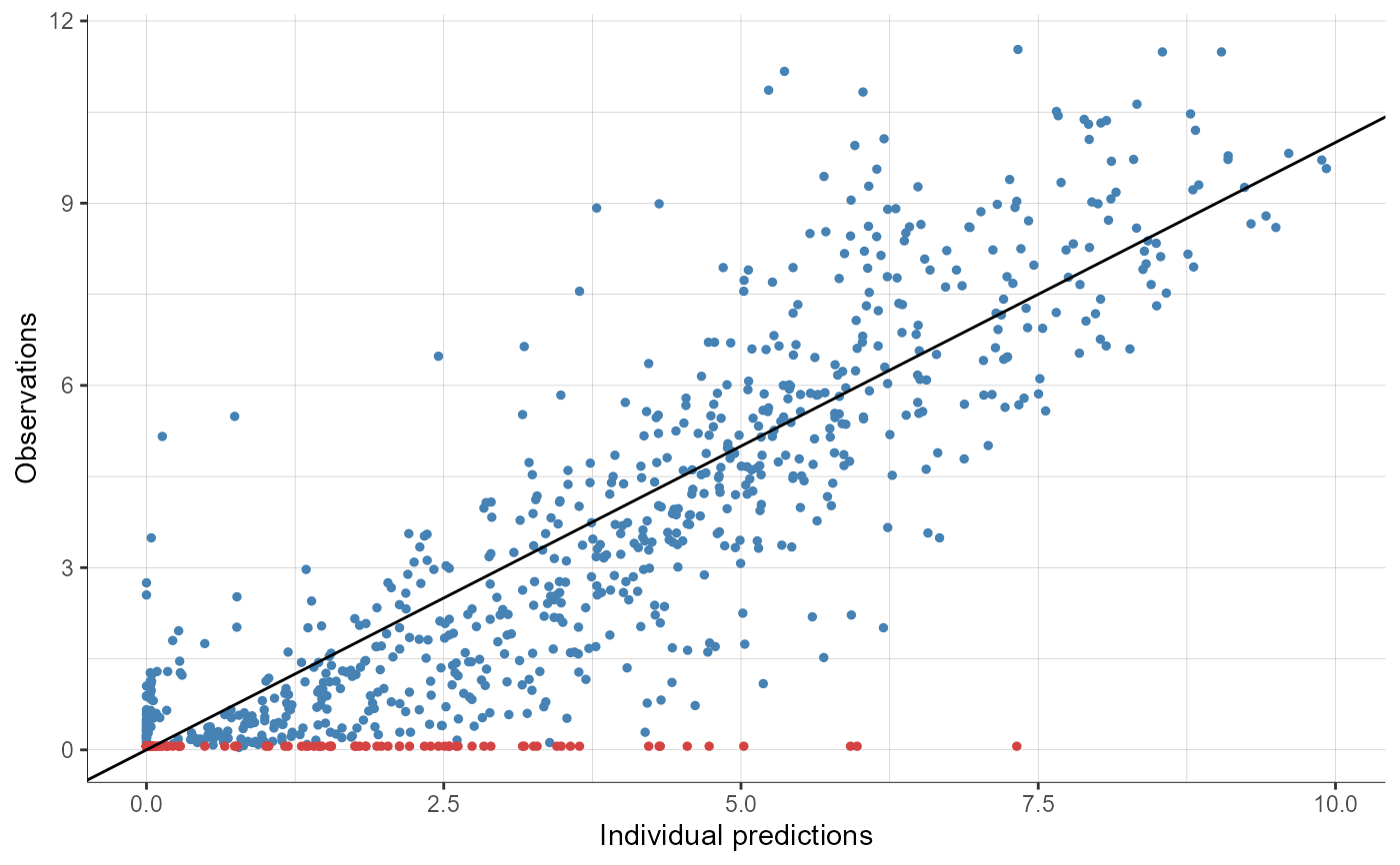
# plot with default options
plotCAObservationsVsPredictions()
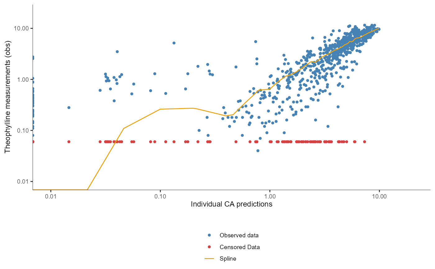
# changing the elements to display
plotCAObservationsVsPredictions(settings=list(spline=T,
                                              useCensored=T,
                                              cens=T,
                                              identityLine=F,
                                              legend=T,
                                              grid=F,
                                              xlog=T,
                                              ylog=T,
                                              xlim=c(0.01,20),
                                              ylim=c(0.01,20),
                                              fontsize=9,
                                              xlab=c('Individual CA predictions'),
                                              ylab=c('Theophylline measurements (obs)')))
#> Warning: log-10 transformation introduced infinite values.
#> Warning: log-10 transformation introduced infinite values.
#> Warning: NaNs produced
#> Warning: log-10 transformation introduced infinite values.
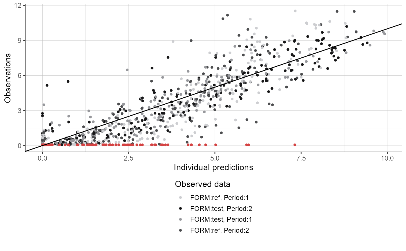
# coloring by FORM and Period using a greyscale
plotCAObservationsVsPredictions(settings = list(legend=T),
                                stratify = list(color=c("FORM", "Period"),
                                                colors=c("#cdced1","#97989c","#4c4d4f","#161617")))
# coloring by FORM and filtering to keep only SEQ=TR
plotCAObservationsVsPredictions(settings = list(legend=T),
                                stratify = list(color=c("FORM"),
                                                filter=list("SEQ","TR")))
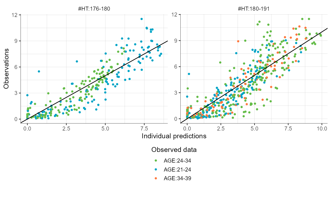
# defining groups for AGE and HT, coloring by AGE and splitting by HT
plotCAObservationsVsPredictions(settings = list(legend=T, cens=F),
                                stratify = list(groups=list(list(name="AGE", definition=c(24, 34)),
                                                            list(name="HT", definition=180)),
                                                color="AGE",
                                                colors=c("#00a4c6","#64bc48","#ff793f"),
                                                split="HT"))