plotCAIndividualFits

Plot the CA individual fits.

Usage

        R
    
plotCAIndividualFits(
  obsName = NULL,
  settings = list(),
  preferences = list(),
  stratify = list()
)

Arguments

obsName

(character) Name of the observation (if several OBS ID are used). By default the first observation is considered.

settings

List with the following settings:

obsDots (logical) - If TRUE, individual observations are displayed as dots (default TRUE).
obsLines (logical) - If TRUE, individual observations are displayed as lines (default FALSE).
cens (logical) - If TRUE, censored observations are displayed as intervals (default TRUE).
indivFits (logical) - If TRUE, individual fits are displayed (default TRUE).
dosingTimes (logical) - If TRUE, dosing times are displayed as vertical lines (default FALSE).
splitOccasions (logical) - If TRUE, occasions are displayed on separate subplots (default TRUE). If FALSE, all occasions are overlaid on the same subplot.
legend (logical) If TRUE, plot legend is displayed (default FALSE).
grid (logical) If TRUE, plot grid is displayed (default TRUE).
xlog (logical) If TRUE, log-scale on x axis is used (default FALSE).
ylog (logical) If TRUE, log-scale on y axis is used (default FALSE).
xlab (character) label on x axis (default "time").
ylab (character) label on y axis (default: observation name).
ncol (integer) number of columns to arrange the subplots (default 4).
xlim (c(double, double)) limits of the x axis.
ylim (c(double, double)) limits of the y axis.
fontsize (integer) Font size of text elements (default 11).
units (logical) If TRUE, units are added in axis labels (default TRUE).
scales (character) Should scales be fixed ("fixed"), free ("free", default), or free in one dimension ("free_x", "free_y").

preferences

(optional) preferences for plot display, run getPlotPreferences("plotCAIndividualFits") to check available displays.

stratify

List with the stratification arguments. Stratification is not available in case "sparse data" calculations are used.

groups - Definition of stratification groups. By default, stratification groups are already defined as one group for each category for categorical covariates and occasions, and two groups of equal number of individuals for continuous covariates. To redefine groups, for each covariate to redefine, specify a list with:

`name`	(character)	covariate name (e.g `"AGE"`)
`definition`	(vector(continuous) \|\| list>(categorical))	For continuous covariates, vector of break values (e.g `c(35, 65)`). For categorical covariates, groups of categories as a list of vectors (e.g `list(c("study101"), c("study201","study202"))`)

filter (list< list> >) - List of pairs containing a covariate name and the vector of indexes or categories (for categorical covariates) of the groups to keep (by default no filtering is applied). For instance, list("AGE",c(1,3)) to keep the individuals belonging to the first and third age group, according to the definition in groups. For instance, list("FORM","ref") using the category name for categorical covariates.
color (vector) - Vector of covariates used for coloring (by default no coloring is applied). For instance c("FORM","AGE").
colors - Vector of colors to use when color argument is used. Takes precedence over colors defined in preferences. For instance c("#ebecf0","#cdced1","#97989c").
individualSelection - Ids to display (by default the 12 first ids are displayed) defined as:
- indices (vector) - Indices of the individuals to display (by default, the 12 first individuals are selected). If occasions are present, all occasions of the selected individuals will be displayed. Takes precedence over ids. For instance c(5,6,10,11).
- isRange (logical) - If TRUE, all individuals whose index is inside [min(indices), max[indices]] are selected (FALSE by default). Forced to FALSE if ids is defined.
- ids (vector) - Names of the individuals to display. If occasions are present, all occasions of the selected individuals will be displayed. For instance c("101-01","101-02","101-03"). If ids are integers, can also be c(1,3,6). Ignored if indices is defined.

Value

A ggplot object

Examples

R

  initializeLixoftConnectors(software = "pkanalix")
  project <- file.path(getDemoPath(), "/2.case_studies/project_Theo_extravasc_SD.pkx")
  loadProject(project)
  runCAEstimation()
  
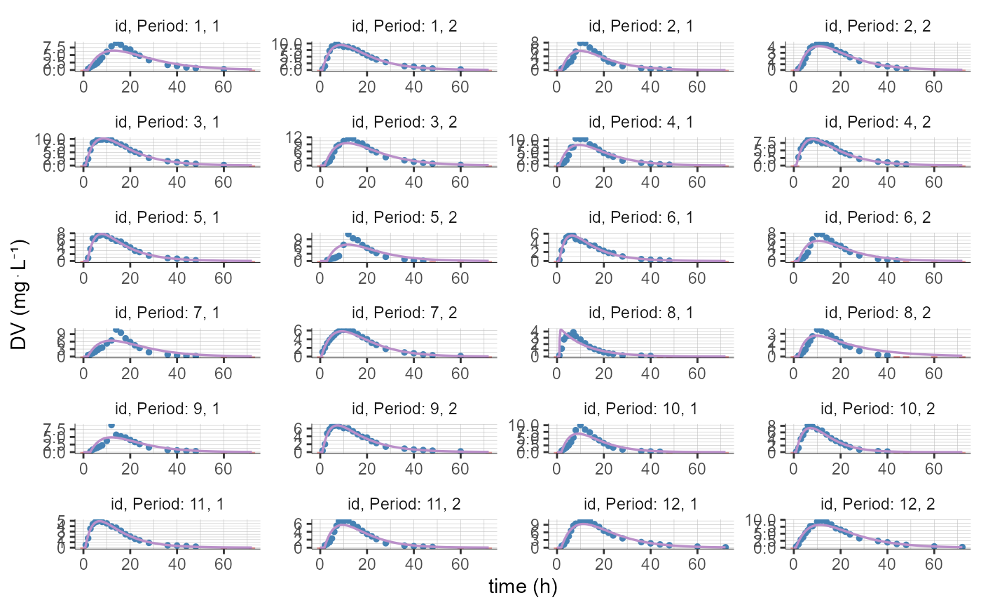
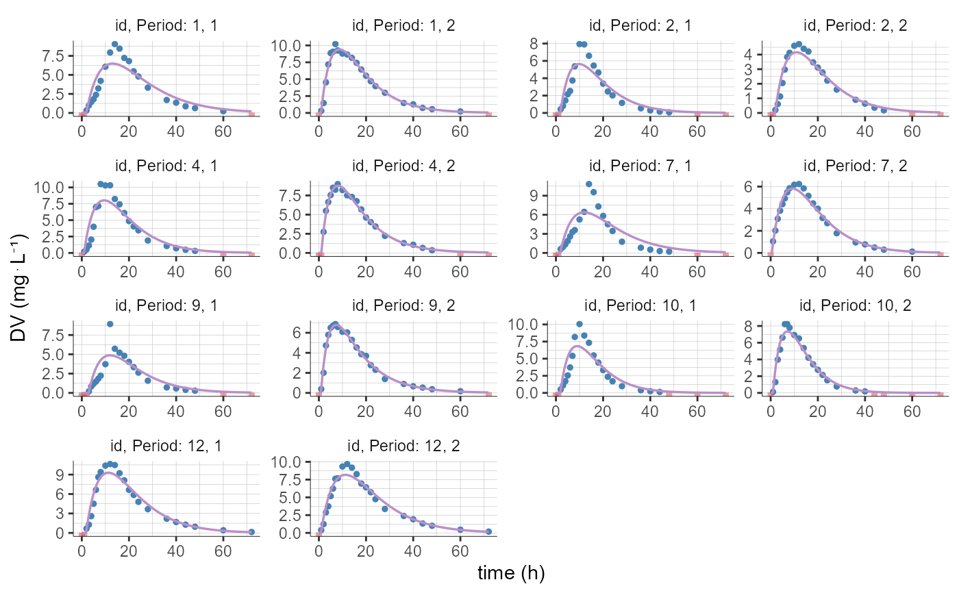
# by default 12 individuals are displayed (with 2 occasions each in this example)
plotCAIndividualFits()
#> Warning: No shared levels found between `names(values)` of the manual scale and the
#> data's fill values.
#> Warning: No shared levels found between `names(values)` of the manual scale and the
#> data's linetype values.

R



# loop to create several plots ("pages") with 6 individuals (2 occasions each) per page, using "indices" and "isRange"
nbIndiv <- 18
nbIndivPerPage <- 6
nbPages <- ceiling(nbIndiv/nbIndivPerPage)
for(i in 1:nbPages){
  plotCAIndividualFits(stratify = list(individualSelection=list(indices=c(nbIndivPerPage*(i-1)+1,nbIndivPerPage*i),
                                                                isRange=T)))
}

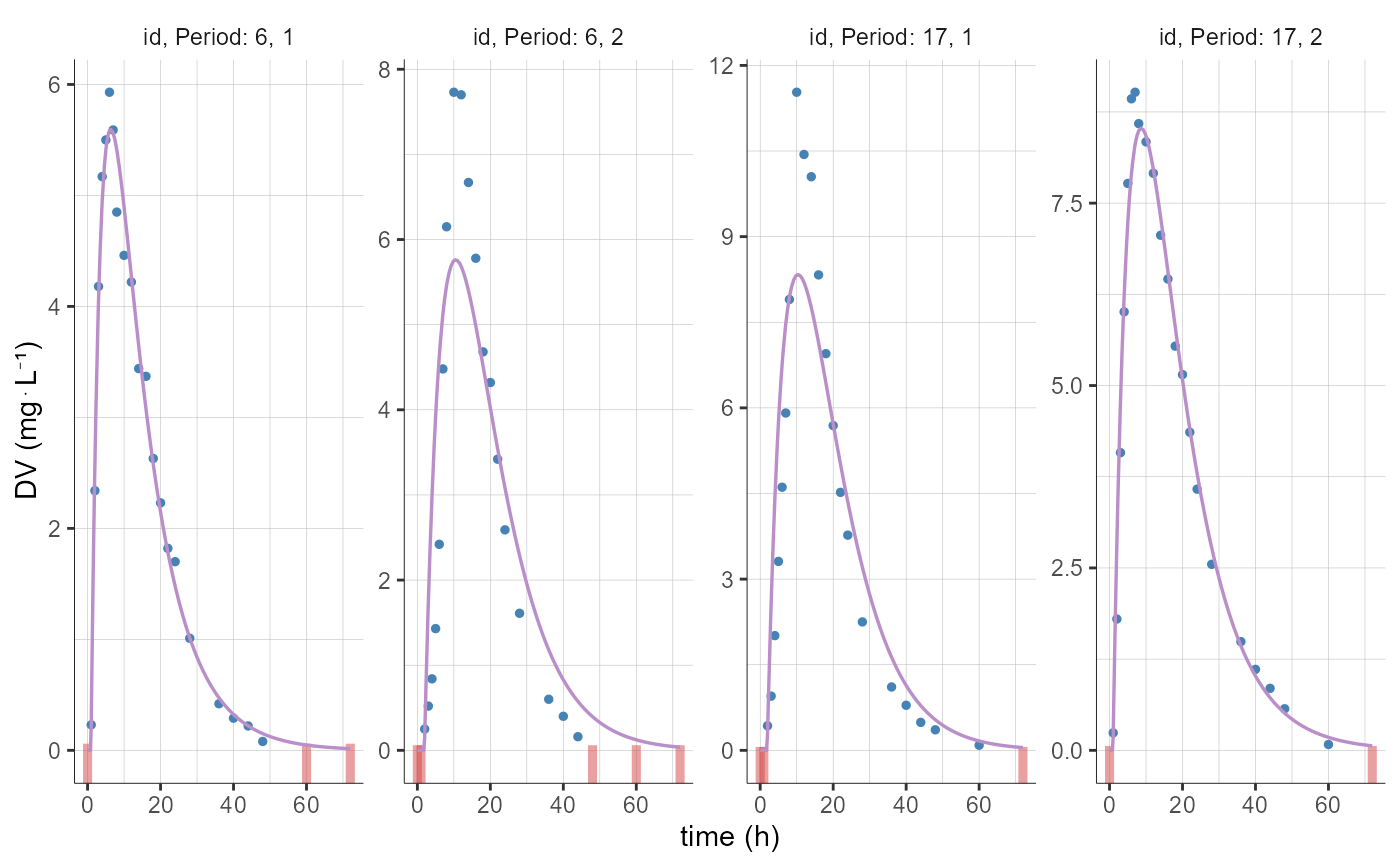
# selection of individuals based on id names
plotCAIndividualFits(stratify = list(individualSelection=list(ids=c("6","17"))))
#> Warning: No shared levels found between `names(values)` of the manual scale and the
#> data's fill values.
#> Warning: No shared levels found between `names(values)` of the manual scale and the
#> data's linetype values.

R


plotCAIndividualFits(stratify = list(individualSelection=list(ids=c(6, 17))))
#> Warning: No shared levels found between `names(values)` of the manual scale and the
#> data's fill values.
#> Warning: No shared levels found between `names(values)` of the manual scale and the
#> data's linetype values.

R




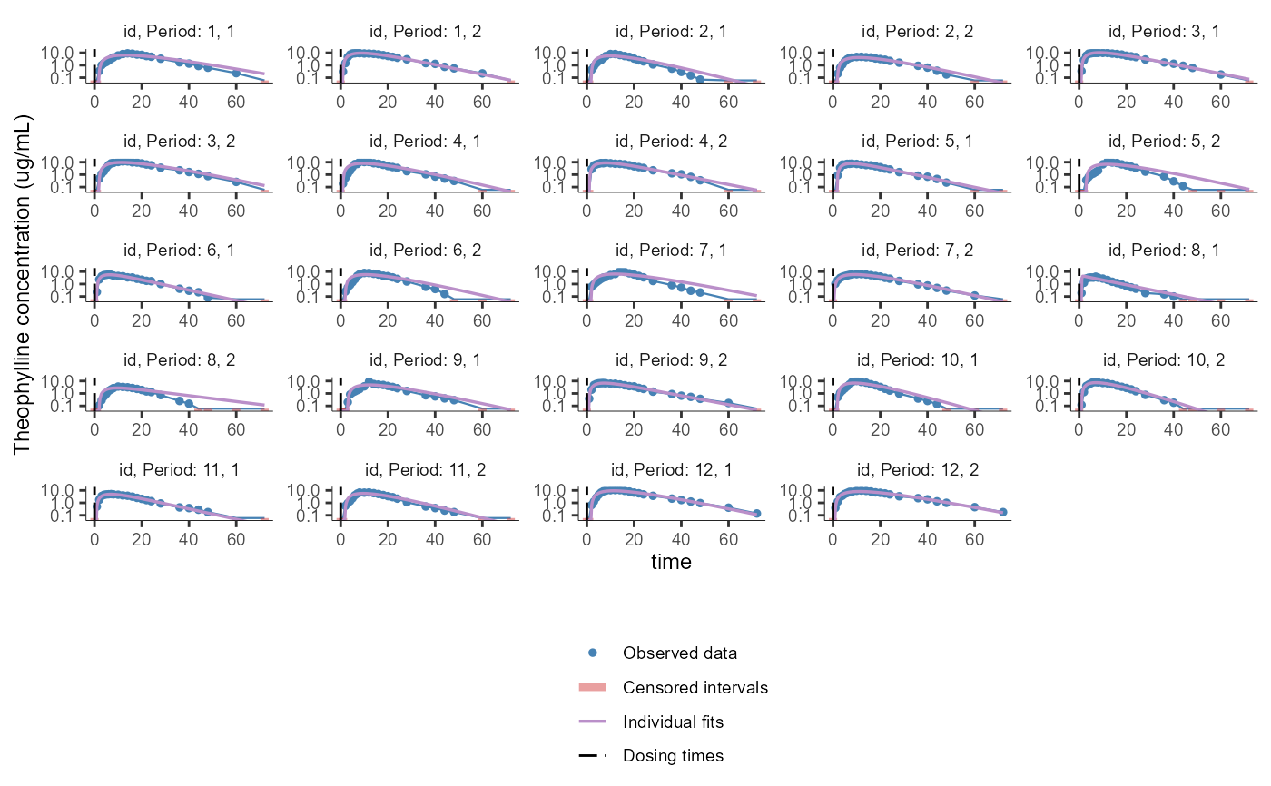
# changing the elements to display
plotCAIndividualFits(settings = list(obsDots=T, 
                                     obsLines=T, 
                                     cens=T,
                                     dosingTimes=T,
                                     splitOccasions=T, 
                                     ncol=5, 
                                     legend=T, 
                                     grid=F, 
                                     ylog=T,
                                     units=F, 
                                     fontsize=9,
                                     ylim=c(0.05,15),
                                     ylab="Theophylline concentration (ug/mL)"))
#> Warning: NaNs produced
#> Warning: log-10 transformation introduced infinite values.
#> Warning: No shared levels found between `names(values)` of the manual scale and the
#> data's fill values.
#> Warning: No shared levels found between `names(values)` of the manual scale and the
#> data's linetype values.

R



# get available preferences
getPlotPreferences("plotCAIndividualFits")
#> $obs
#> $obs$color
#> [1] "#4682B4"
#> 
#> $obs$radius
#> [1] 1
#> 
#> $obs$shape
#> [1] 19
#> 
#> $obs$lineWidth
#> [1] 0.4
#> 
#> $obs$lineType
#> [1] "solid"
#> 
#> $obs$legend
#> [1] "Observed data"
#> 
#> 
#> $censObsIntervals
#> $censObsIntervals$color
#> [1] "#D44242"
#> 
#> $censObsIntervals$opacity
#> [1] 0.5
#> 
#> $censObsIntervals$lineType
#> [1] "solid"
#> 
#> $censObsIntervals$lineWidth
#> [1] 1.6
#> 
#> $censObsIntervals$legend
#> [1] "Censored intervals"
#> 
#> 
#> $indivFits
#> $indivFits$color
#> [1] "#BA8FC9"
#> 
#> $indivFits$lineWidth
#> [1] 0.6
#> 
#> $indivFits$lineType
#> [1] "solid"
#> 
#> $indivFits$legend
#> [1] "Individual fits"
#> 
#> 
#> $dosingTimes
#> $dosingTimes$color
#> [1] "#000000"
#> 
#> $dosingTimes$lineWidth
#> [1] 0.5
#> 
#> $dosingTimes$lineType
#> [1] "longdash"
#> 
#> $dosingTimes$legend
#> [1] "Dosing times"
#> 
#> 

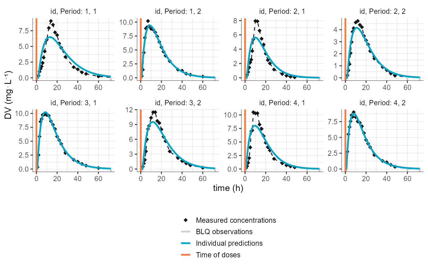
# change color, radius, shape, lineType, lineWidth and legend for all elements
plotCAIndividualFits(settings = list(legend=T, obsLines=T, dosingTimes=T),
                     stratify = list(individualSelection=list(ids=c(1,2,3,4))),
                     preferences = list(obs=list(color="#161617",
                                                 radius=2,
                                                 shape=18,
                                                 lineWidth=0.5,
                                                 lineType="dashed",
                                                 legend="Measured concentrations"),
                                        censObsIntervals=list(color="#cdced1",
                                                              opacity=1,
                                                              lineType="solid",
                                                              lineWidth=1,
                                                              legend="BLQ observations"),
                                        dosingTimes=list(color="#ff793f",
                                                         lineWidth=1,
                                                         lineType="solid",
                                                         legend="Time of doses"),
                                        indivFits=list(color="#00a4c6",
                                                       lineWidth=1,
                                                       lineType="solid",
                                                       legend="Individual predictions")))
#> Warning: No shared levels found between `names(values)` of the manual scale and the
#> data's fill values.
#> Warning: No shared levels found between `names(values)` of the manual scale and the
#> data's linetype values.

R



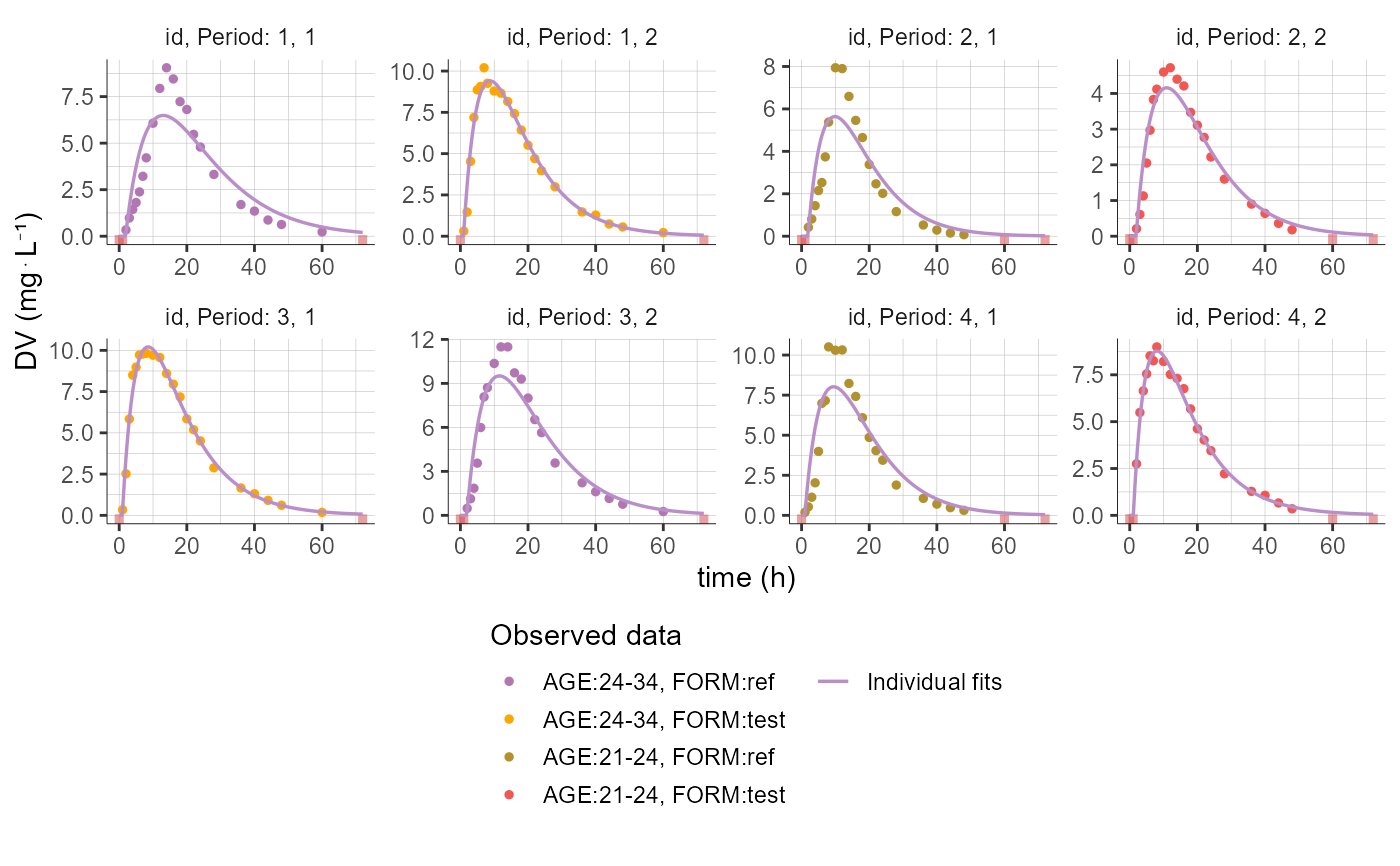
# define groups for AGE and color by AGE and FORM
plotCAIndividualFits(settings=list(legend=T),
                     stratify = list(groups=list(name="AGE", definition=c(24, 34)),
                                     color=c("AGE","FORM"),
                                     individualSelection=list(ids=c(1,2,3,4))))
#> Warning: No shared levels found between `names(values)` of the manual scale and the
#> data's fill values.

R



# filter to keep only individuals with sequence "RT" (first among "RT" and "TR")
plotCAIndividualFits(stratify = list(filter=list(list("SEQ","RT"))))
#> Warning: No shared levels found between `names(values)` of the manual scale and the
#> data's fill values.
#> Warning: No shared levels found between `names(values)` of the manual scale and the
#> data's linetype values.

R


plotCAIndividualFits(stratify = list(filter=list(list("SEQ",1))))
#> Warning: No shared levels found between `names(values)` of the manual scale and the
#> data's fill values.
#> Warning: No shared levels found between `names(values)` of the manual scale and the
#> data's linetype values.

R

$body

plotCAIndividualFits

[PKanalix] Generate CA Fit plots

Usage

Arguments

Value

See also

Examples