Using or editing models from the libraries

Nine different libraries are available in Monolix, detailed in Libraries of models

PK (pharmacokinetics)
PD (pharmacodynamics)
PKPD (joint PKPD)
PK double absorption
Parent metabolite
TMDD (target-mediated drug disposition)
TTE (time to-event)
Count (for non-continuous count data)
TGI (tumor growth and tumor growth inhibition)

Picking a model from a library

To use a model from the libraries, in the Structural model tab, click on “Load from library” and select the desired library. A list of models appears, as well as a menu to filter them. Use the filters and the list of parameters included in the models to select the model you need.

Here is for example how to select a PK model with first-order absorption and linear elimination (parameters ka, V, Cl):

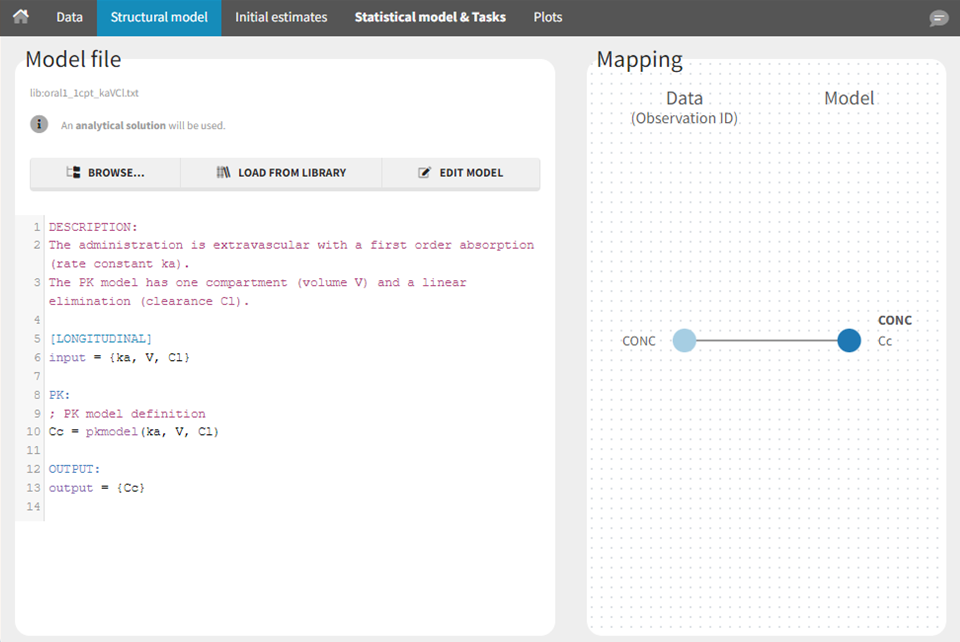
The model contents correspond to pre-written models in Mlxtran language. In the case of library models, they are not saved as external text files but are generated on-the-fly inside Monolix. Once selected, the model appears in the Monolix GUI. Below we show the content of the (ka,V,Cl) model:

https://www.youtube.com/watch?v=Ojy9kII5Ylo

Modifying a model from the libraries

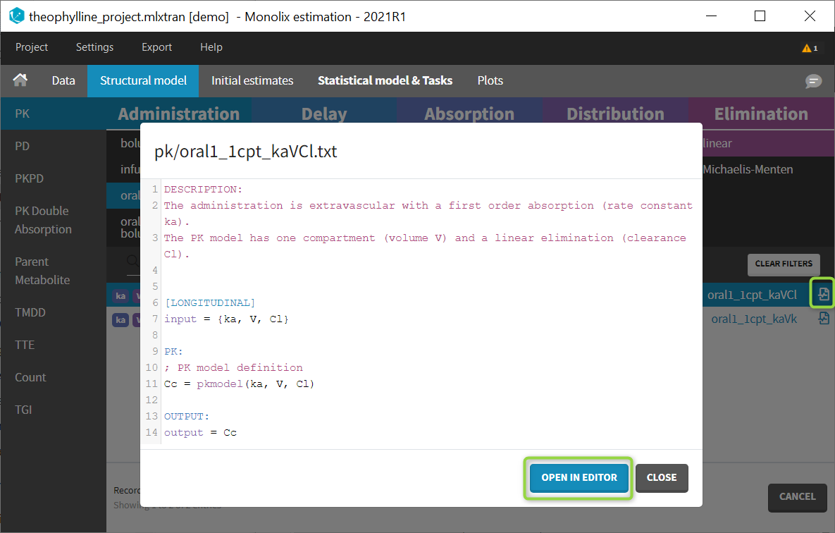
Browse existing models from the libraries using the “Load from library” button, then click the “file” icon next to a model name. This opens a pop-up window where the content of the model file is displayed. Click on “Open in editor” to open the model file in the MlxEditor. There you can adapt the model, for instance to add a PD model. Be careful to save the new model under a new name, to avoid overwriting the library files.

The video below shows an example of how a scale factor can be added to a library model:

https://www.youtube.com/watch?v=qzbae1S7cik

The video below shows how to combine several library models together:

https://youtu.be/5r_7_Z1bWq8?si=qEF6FwLYxtWM68Ix

Step-by-step example with the PK library

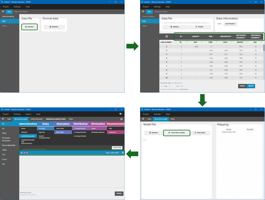
We would like to set up a one compartment PK model with first order absorption and linear elimination for the theophylline data set. We start by creating a new Monolix project. Next, in the Data tab, click browse, and select the theophylline data set. In this example, all columns are already automatically tagged, based on the header names. We click ACCEPT and NEXT and arrive on the Structural model tab, click on LOAD FROM LIBRARY to choose a model from the PK library. The menu at the top allow to filter the list of models: after selecting an oral/extravascular administration, no delay, first-order absorption, one compartment, a linear elimination and parametrization with clearance, one model remains in the list, with parameters (ka,V,Cl). Click on the oral1_1cpt_kaVCl model to select it.

After this step, the GUI moves to the Initial Estimates tab, but it is possible to go back to the Structural model tab to see the content of the file:

CODE

[LONGITUDINAL]
input = {ka, V, Cl}

EQUATION:
Cc = pkmodel(ka, V, Cl)

OUTPUT:
output = Cc

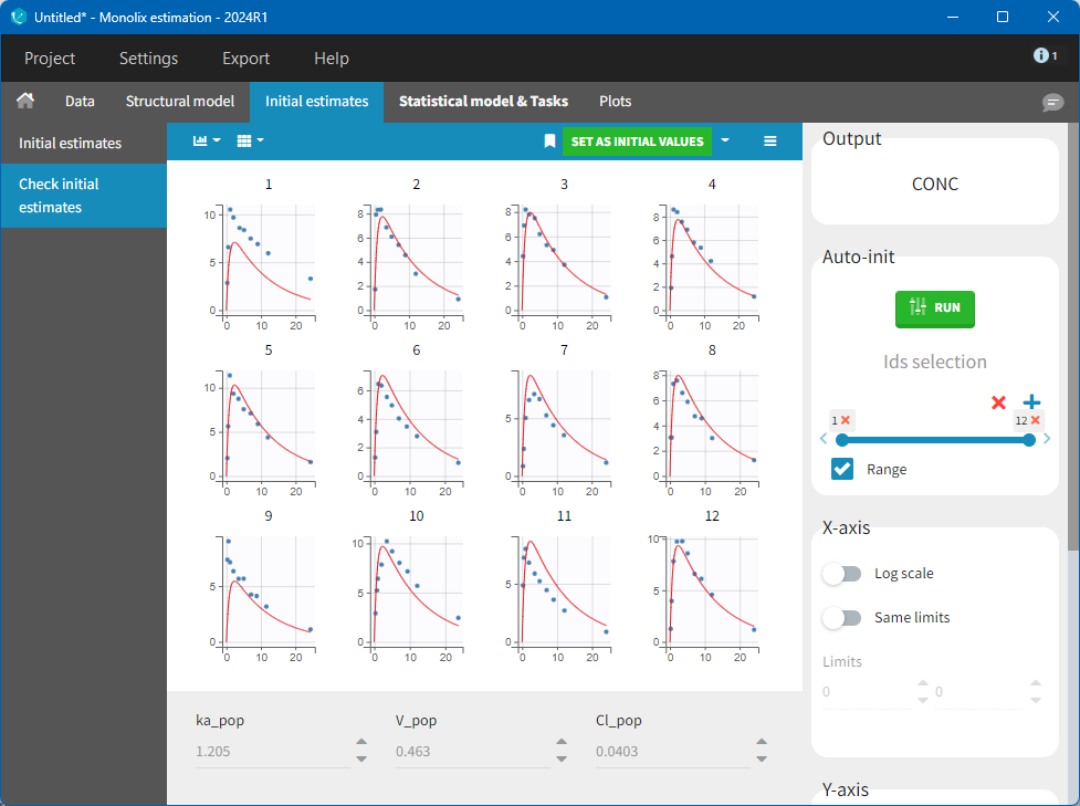
Back to the Initial Estimates tab, the initial values of the population parameters can be adjusted by comparing the model prediction using the chosen population parameters and the individual data. Click on SET AS INITIAL VALUES when you are done.

In the next tab, the Statistical model & Tasks tab, Monolix uses by default:

A combined error observation model
Lognormal distributions for all parameters (ka, V and Cl)

At this stage, the monolix project should be saved. This creates a human-readable text file with extension .mlxtran, which contains all the information defined via the GUI. In particular, the name of the model appears in the section [LONGITUDINAL] of the saved project file:

CODE

<MODEL>
[INDIVIDUAL]
input = {ka_pop, omega_ka, V_pop, omega_V, Cl_pop, omega_Cl}

DEFINITION:
ka = {distribution=lognormal, typical=ka_pop, sd=omega_ka}
V = {distribution=lognormal, typical=V_pop, sd=omega_V}
Cl = {distribution=lognormal, typical=Cl_pop, sd=omega_Cl}

[LONGITUDINAL
input = {a, b}
file = 'lib:oral1_1cpt_kaVCl.txt'

DEFINITION:
CONC = {distribution=normal, prediction=Cc, errorModel=combined1(a,b)}