
Drugs can undergo a transformation into metabolites – pharmacologically active and/or producing adverse effects. They can impact the pharmacokinetics of the parent and drive the efficacy. But, at the same time, can rise safety concerns. Joint parent – metabolite models account for the impact of the parent-metabolite interactions on the estimation.
The library of Parent – Metabolite models built-in the MonolixSuite includes many characteristic mechanisms, such as first pass effect, uni and bidirectional transformation and up to three compartments for parent and metabolite, which makes it an excellent tool for exploration and modeling. The implementation with mlxtran macros uses analytical solutions for faster parameter estimation and makes a great basis for the development of more complex models.
Administration
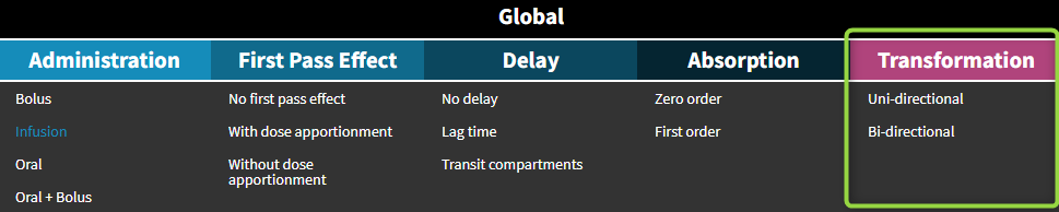
Select administration route, delay, absorption mechanism and first pass effect to correctly model drug input. |
Transformation
Check non-reversible and reversible metabolic systems to predict the impact of parent-metabolite interactions. |
Distribution
Explore different number of peripheral compartments independently for parent and metabolite. |
Elimination
Try linear or non-linear Michaelis-Menten elimination mechanism to get a better fit. |
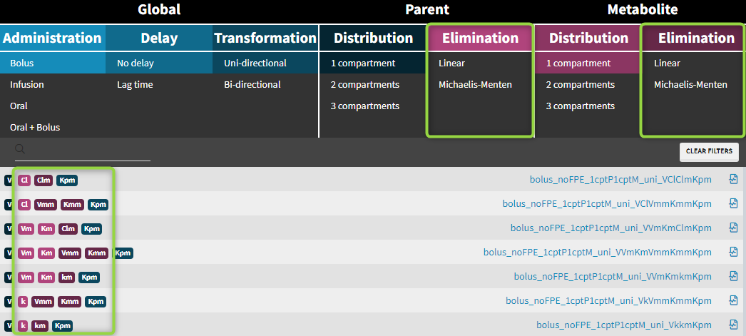
Parent-metabolite model filters
Administration
Parent-metabolite models can be combined with standard administration routes: bolus, infusion, oral/extravascular and oral with bolus.
Intravenous doses (bolus, infusion) are always administered to the central parent compartment, can be with or without a time delay and do not include the first pass effect.
Oral doses can be with the following options:
-
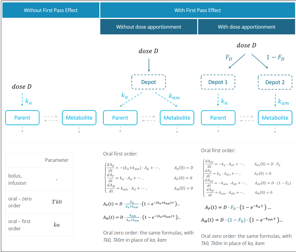
with or without the first pass effect: with first pass effect, doses are split between parent and metabolite, either with dose apportionment Fd or without dose apportionment (see more details below)
-
zero (Tk0) or first order absorption process (ka for parent, kam for metabolite in case of the first pass effect)
-
without or with a time delay (Tlag) or with transit compartments (Mtt, Ktr)
-
oral + bolus: bioavailability F (estimated as a separated parameter)
First pass effect
The first pass effect is a phenomenon in which a drug undergoes any biotransformation at a specific location in the body – for example transformation of parent to metabolite before reaching its site of action or the systemic circulation. The first-pass effect can be clinically relevant when the metabolized fraction is high or when it varies significantly from individual to individual or within the same individual over time, resulting in variable or erratic absorption. It also has an impact on peak drug concentrations, which may result in parent concentration peaks occurring much earlier.
In the Monolix library, models with the first pass effect include splitting a dose – with or without dose apportionment – and absorbing one fraction in the central parent compartment (Tk0 or ka) and the other fraction in the central metabolite compartment (Tk0m or kam). The absorption process, zero or first order, is the same for parent and metabolite.
-
Dose apportionment means that the splitting is independent of the absorption constants (Tk0, Tk0m or ka, kam), with a fraction Fd of the dose leading to the parent and a fraction 1 – Fd leading to the metabolite prior to reach the plasma.
-
In models without dose apportionment, dose splitting is implicit and results from different absorption rates ka, kam (or absorption times Tk0, Tk0m).
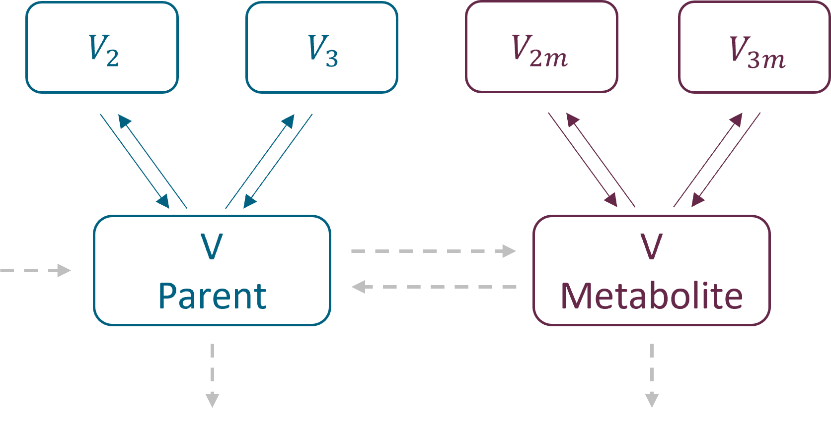
Distribution
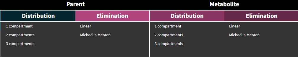
In the library it is possible to select different number of compartments for parent and for metabolite. The central compartments have the same volume V – identifiability issue when only parent drug is administered.
Parametrization
Parent and metabolite have the same parametrization. As for the PK and PKPD libraries, there are two parametrizations available:
-
with exchange rates: k12, k21 for parent and k12m, k21m for metabolite for the second compartments, and k13, k31 and k13m, k31m for the third compartments. Peripheral compartments are defined implicitly through the exchange rates, so volumes V2, V3, V2m and V3m are not needed in the model. The volume of central compartments is V (for both parent and metabolite)
-
with inter – compartment clearance: Q2, V2, Q3, V3 for parent and Q2m, V2m, Q3m, V3m for metabolite. The volume of central compartments is V1 (for both parent and metabolite), to be compatible with the PK models in case of the sequential model development.
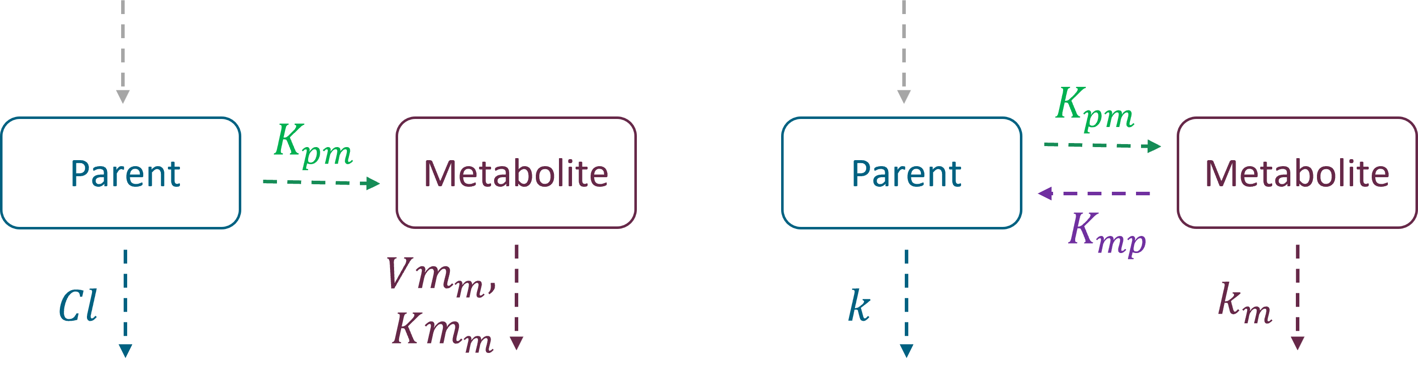
Transformation and elimination
The parent drug, after administration, is eliminated from the system or transformed into a metabolite, which subsequently is also eliminated. In addition, the metabolite can be back-transformed into the parent drug – it is a common process for example for amines. Both unidirectional and reversible transformations can be selected from the “global” section of filters in the library. The elimination, linear or non-linear (Michaelis-Menten), is specific for parent and for metabolite.
-
Transformation:
-
Kpm – transformation rate from parent to metabolite
-
Kmp – transformation rate from metabolite to parent
-
-
Elimination: parent and metabolite can be eliminated with different process (linear or non-linear)
-
Cl, k, Vm, Km – elimination parameters for parent
-
Clm, km, Vmm, Kmm – elimination parameters for metabolite
-
Examples:
Analytical solutions
Implementation in the Mlxtran
Example 1: a model with oral absorption (rate ka) of a dose D, one central compartment for parent (cmt = 1) and one for metabolite (cmt = 2), linear elimination (rates: k, km) and uni-directional transformation (rate Kpm), is the following:

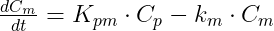
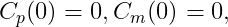
where Cp and Cm are the concentrations in the central compartments of parent and metabolite respectively.
Models in the parent-metabolite Monolix library are built using mlxtran macros. For the above model:
;PK model definition for parent
compartment(cmt = 1, volume = V, concentration = Cp)
oral(cmt = 1, ka)
elimination(cmt = 1, k)

;PK model definition for metabolite
compartment(cmt = 2, volume = V, concentration = Cm)
elimination(cmt = 2, k = km)
transfer(from = 1, to = 2, kt = Kpm)
Example 2:
You can see in the collapsable sections just below the model corresponding to 1s-order oral absorption with lag time, two compartments (central and peripheral) for both parent and metabolite, linear eliminations and uni-directional transformation. The 1st version is written with PK macros and is the one implemented in the library, it is advised to use that one as it makes use of the analytical solutions. The 2nd version is the same model written with ODEs.
Analytical solutions
Analytical solutions, which are more accurate than numerical solutions and are faster than ODE solvers, are implemented for parent – metabolite models satisfying the following conditions:
-
administration (bolus, IV, oral 0 or 1st order) is to the central parent compartment only => models from the library with first pass effect (“with dose apportionment” and “without dose apportionment”) do not use analytical solutions
-
parameters are not time-dependent (exception: dose coefficients such as Tlag, which are evaluated only once),
-
the elimination is linear and only from the central parent and/or the metabolite compartments, => models from the library with elimination = “Michaelis-Menten” do not use the analytical solutions
-
there are no transit compartments, => models from the library with delay = “transit compartments” do not use the analytical solution
-
the transfer between parent and metabolite is only between their central compartments,
-
there are maximally two peripheral compartments for parent and maximally two for metabolite.
Comparison of the performance between analytical and numerical solutions
The following example compares the computational time (in seconds) of the parameter estimation task (SAEM) using analytical solutions (AS) and numerical solutions (ODE) for models with different number of compartments.
Dataset: simulated in Simulx N = 100 individuals, who received a single or multi oral doses. 5 or 20 measurements of both, parent and metabolite concentrations registered for each individual.
SAEM: (fixed number of iterations) 500 iterations for the exploratory phase, 200 iterations for the smoothing phase.
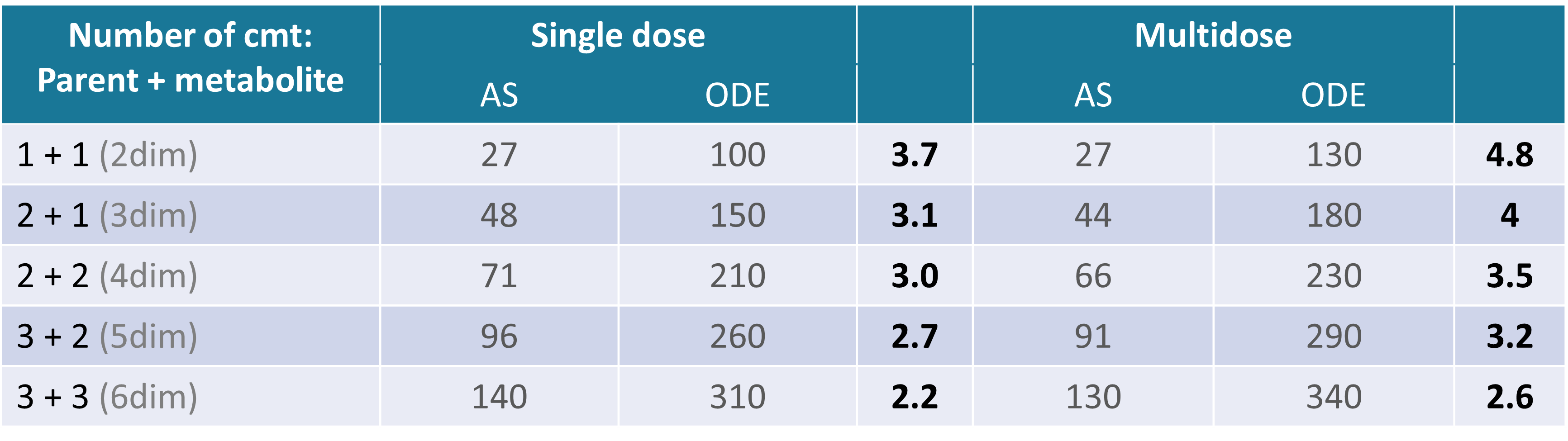
Times are given in seconds, and values in bold give the speed up ratio when using an analytical solution.