To run the examples below, Monolix and Simulx projects are provided with the mlxDesignEval R package. The path to these files can be obtained using
proj <- system.file("extdata","theophylline_project.mlxtran", package="mlxDesignEval"). We will use this syntax for most examples.
First example
Evaluating the design
To perform a design evaluation, you need to call the evaluate_design() function and define as input arguments the model and the design. The model can be provided as a Monolix or Simulx project (in the project_file argument), or as a model file in mlxtran syntax (in the model_file argument). The population parameters values are either read from the Monolix or Simulx project, or defined via the argument population_parameters. The design is provided in the arguments output, treatment and group, as well as covariate, regressor and occasion if needed.
In the example below, we show a basic call using the following arguments:
-
project_file: the Monolix theophylline project containing a simple 1-compartment model with parameters (ka, V, Cl)
-
population_parameters: the population parameter values defined as a data frame which gives the typical population values (e.g V_pop), the standard deviation of the random effects representing the inter-individual variability (omega_V), and the error model parameters (a and b)
-
output: the planned measurement times defined as a list with the variable name “CONC” (representing the concentration with residual error) and the times as a data frame
-
treatment: the planned treatment as a list containing a data frame with the dose time and amount
-
group: the number of individuals of the trial defined as a list
-
saved_project: file path and name of the Monolix project to save. Saving the final Monolix project is only necessary if you want to plot the results.
res0a<-evaluate_design(project_file = system.file("extdata","theophylline_project.mlxtran", package="mlxDesignEval"),
                       population_parameters = data.frame(ka_pop=1.5,V_pop=0.45,Cl_pop=0.04, omega_ka=0.66, omega_V=0.12, omega_Cl=0.27, a=0.43, b=0.055),
                       output = list(output="CONC", data=data.frame(time=c(0.25, 0.5, 0.75, 2, 3.5, 6, 8, 12, 24))),
                       treatment = list(data=data.frame(time=0, amount=5)),
                       group = list(size=20),
                       saved_project = "ex0a_saved_project.mlxtran")
The function returns a list containing the expected RSEs on all parameters, the FIM and the objective function value (OFV). The RSEs are expressed as a percentage and represent the uncertainty we expect on the parameters if we would run a trial and estimate the model parameters on the trial data. Larger values represent larger uncertainty. The OFV summarizes the information the design provides. A higher OFV means a more informative design.
print(res0a)
#> $RSE
#>                RSE
#> ka_pop   15.299379
#> V_pop     3.326124
#> Cl_pop    6.432744
#> omega_ka 16.755274
#> omega_V  24.031851
#> omega_Cl 17.869401
#> a        27.390176
#> b        38.241858
#>
#> $OFV
#> [1] 54.73412
#>
#> $FIM
#>             ka_pop      V_pop       Cl_pop    omega_ka     omega_V     omega_Cl
#> ka_pop    19.26120  -34.21355     34.67569  0.00000000    0.000000   0.00000000
#> V_pop    -34.21355 4553.57655   2040.65135  0.00000000    0.000000   0.00000000
#> Cl_pop    34.67569 2040.65135 152084.51566  0.00000000    0.000000   0.00000000
#> omega_ka   0.00000    0.00000      0.00000 81.81267740    4.224042   0.07713584
#> omega_V    0.00000    0.00000      0.00000  4.22404248 1224.383926   4.37147040
#> omega_Cl   0.00000    0.00000      0.00000  0.07713584    4.371470 431.65686635
#> a          0.00000    0.00000      0.00000  3.73420667   91.273824  23.48407510
#> b          0.00000    0.00000      0.00000 19.56438015  566.559389  76.00446616
#>                    a           b
#> ka_pop      0.000000     0.00000
#> V_pop       0.000000     0.00000
#> Cl_pop      0.000000     0.00000
#> omega_ka    3.734207    19.56438
#> omega_V    91.273824   566.55939
#> omega_Cl   23.484075    76.00447
#> a         469.993658  2422.48827
#> b        2422.488270 14759.05395
Comparison with popED
For the purpose of comparing RSE values to results obtained with other packages such as popED, the RSEs need to be calculated on the variances instead of the standard deviations of the random effects and error model parameters. This can be requested using the argument rse_on_variance=T.
res0b <- evaluate_design(project_file = system.file("extdata","theophylline_project.mlxtran", package="mlxDesignEval"),
                       population_parameters = data.frame(ka_pop=1.5,V_pop=0.45,Cl_pop=0.04, omega_ka=0.66, omega_V=0.12, omega_Cl=0.27, a=0.43, b=0.055),
                       output = list(output="CONC", data=data.frame(time=c(0.25, 0.5, 0.75, 2, 3.5, 6, 8, 12, 24))),
                       treatment = list(data=data.frame(time=0, amount=5)),
                       group = list(size=20),
                       rse_on_variance=T)
print(res0b$RSE)
#>                    RSE
#> ka_pop       15.299379
#> V_pop         3.326124
#> Cl_pop        6.432744
#> var_omega_ka 33.510548
#> var_omega_V  48.063702
#> var_omega_Cl 35.738802
#> var_a        54.780352
#> var_b        76.483715
Another vignette shows an in-depth comparison of the results of popED and mlxDesignEval.
Plotting the design
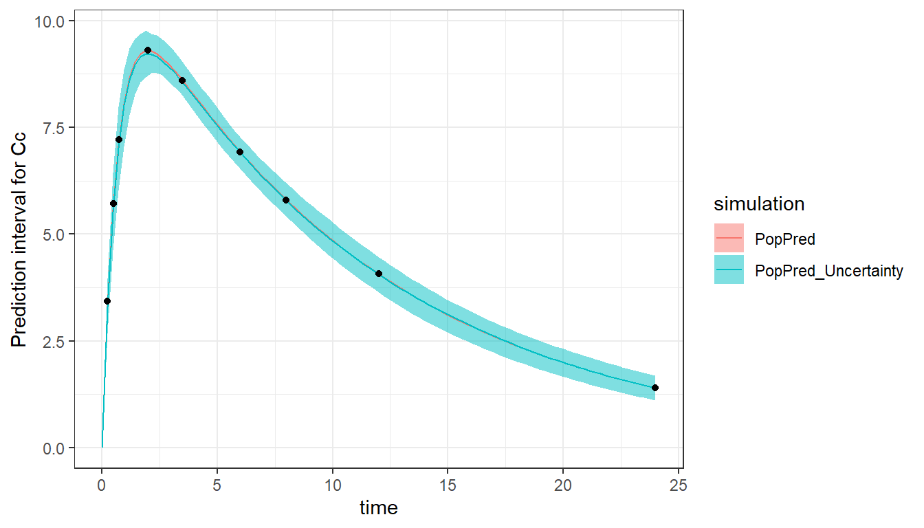
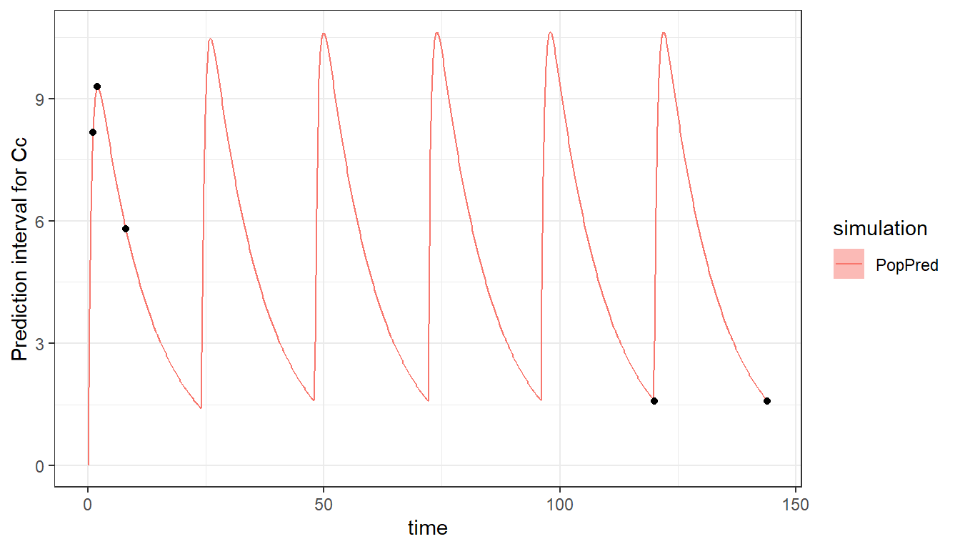
The model can be simulated and plotted in order to check the model and design. To do this, we re-use the Monolix project saved during the evaluate_design() call, as it contains the design information. It is possible to plot the prediction using the population parameters (with plot = c("PopPred")) and/or using sampled individual parameters (with plot = c("IndivPred")). Taking into account the uncertainty of the population parameters is also possible with "PopPred_Uncertainty" and "IndivPred_Uncertainty". The uncertainty is represented by the 90% prediction interval calculated on nrep (by default 100) sets of population parameters sampled from their uncertainty distribution characterized by the RSE (and covariance matrix). Note that it is the smooth prediction (without residual error) which is displayed. The black dots represent the times at which a measurement is planned (corresponding to the output argument of evaluate_design).
plot_prediction(saved_project = "ex0a_saved_project.mlxtran", plot = c("PopPred","PopPred_Uncertainty"))
The “PopPred” line reflects the value of the input population parameters, while the “PopPred_Uncertainty” interval reflects the uncertainty (RSEs) of the population parameters we would obtain with this design.
Comparing designs
In this section, we show how different designs will affect the RSEs.
Dense design
Still using the theophylline project, we first consider a design with 20 individuals and dense sampling after a single dose.
proj <- system.file("extdata","theophylline_project.mlxtran", package="mlxDesignEval")
pop  <- data.frame(ka_pop=1.5,V_pop=0.45,Cl_pop=0.04, omega_ka=0.66, omega_V=0.12, omega_Cl=0.27, a=0.43, b=0.055)
trt  <- list(data=data.frame(time=0, amount=5))
out  <- list(output="CONC", data=data.frame(time=c(0.25, 0.5, 0.75, 2, 3.5, 6, 8, 12, 24, 48)))

res1a<-evaluate_design(project_file          = proj,
                       population_parameters = pop,
                       treatment             = trt,
                       output                = out,
                       group                 = list(size=20),
                       saved_project = "ex1a_saved_project.mlxtran")
This design leads to a good precision of all parameters (RSE<25%).
print(res1a$RSE)
#>                RSE
#> ka_pop   15.291207
#> V_pop     3.310982
#> Cl_pop    6.418395
#> omega_ka 16.747805
#> omega_V  23.835664
#> omega_Cl 17.781250
#> a        14.415191
#> b        24.102536
and an OFV of 56:
print(res1a$OFV)
#> [1] 56.05762
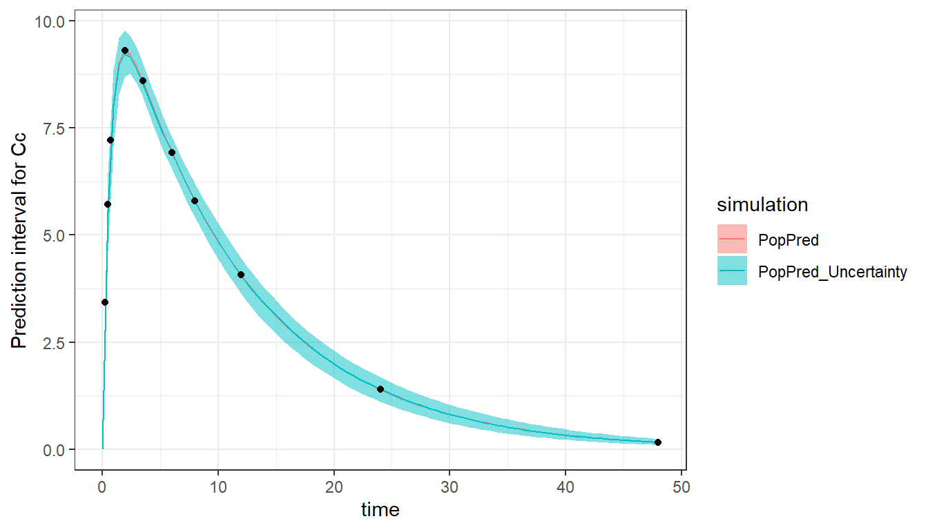
We can visualize the results by plotting the typical population prediction as well as the uncertainty of this prediction (associated to the estimated uncertainty of the population parameters) using 100 sets of sampled population parameters. In this example, as the population parameters have small RSEs, the prediction interval is narrow.
plot_prediction(saved_project = "ex1a_saved_project.mlxtran",
                plot = c("PopPred","PopPred_Uncertainty"),
                nrep = 100)
Sparse design
We next consider a more sparse design with no measurements during the absorption phase:
outSparse <- list(output="CONC", data=data.frame(time=c(3.5, 6, 8, 12, 24, 48)))

res1b <- evaluate_design(project_file          = proj,
                         population_parameters = pop,
                         treatment             = trt,
                         output                = outSparse,
                         group                 = list(size=20),
                         saved_project = "ex1b_saved_project.mlxtran")
With this more sparse design, the RSEs of ka_pop and omega_ka have become large indicating that these parameters will be difficult to estimate using a dataset with measurements after 3.5h only.
print(res1b$RSE)
#>                 RSE
#> ka_pop    99.748033
#> V_pop      4.913990
#> Cl_pop     8.895769
#> omega_ka 302.804840
#> omega_V   32.097400
#> omega_Cl  19.498127
#> a         15.120840
#> b         31.462269
The OFV has decreased from 56 to 44, indicating that this design contains less information than the previous one.
print(res1b$OFV)
#> [1] 44.87338
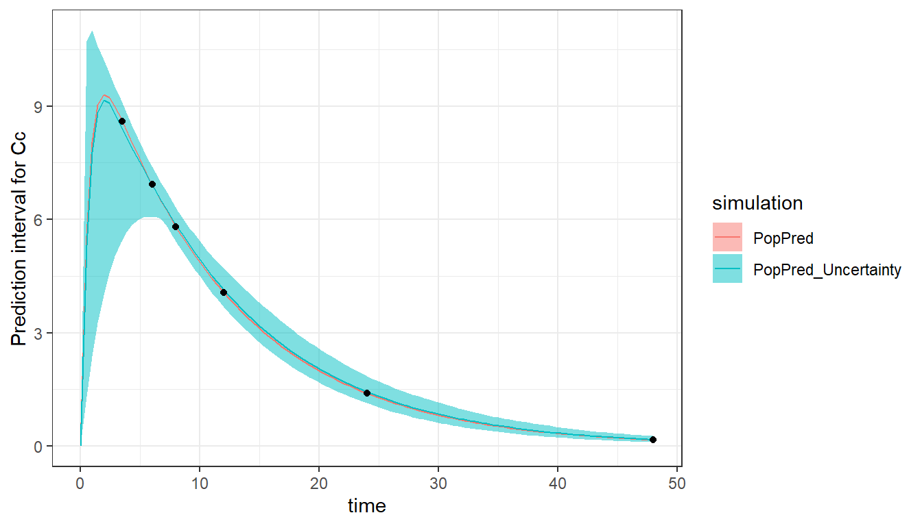
The high uncertainty in the absorption parameters is visible in the prediction interval, which is large during the absorption, where no concentration measurements have been taken.
plot_prediction(saved_project = "ex1b_saved_project.mlxtran",
                plot = c("PopPred","PopPred_Uncertainty"),
                nrep = 100)
More individuals
Going back to the dense design, an even better precision of the population parameters can be obtained by increasing the number of individuals from 20 to 60:
res1c <- evaluate_design(project_file          = proj,
                         population_parameters = pop,
                         treatment             = trt,
                         output                = out,
                         group                 = list(size=60),
                         saved_project = "ex1c_saved_project.mlxtran")
The expected RSEs for a trial with 3 times more individuals are lower:
#>                n20       n60
#> ka_pop   15.291207  8.828380
#> V_pop     3.310982  1.911596
#> Cl_pop    6.418395  3.705658
#> omega_ka 16.747805  9.669338
#> omega_V  23.835664 13.761536
#> omega_Cl 17.781250 10.266003
#> a        14.415191  8.322625
#> b        24.102536 13.915625
Different ways to define the model
Using a Monolix project
A convenient way to define the model is to use a Monolix project, which contains the structural and statistical part (parameter distributions, covariate effects, error model) of the model. The Monolix project can for instance correspond to a run on a pilot study, which is then used to evaluate the best design for a bigger study. Or it can use a dummy dataset and no estimated population parameters, just being a convenient way to define the model. The population parameters can be given separately or read from the Monolix project (if the task “Pop. param.” has run).
We first show an example where the population parameters are provided as a separate argument:
proj1 <- system.file("extdata","theophylline_project.mlxtran", package="mlxDesignEval")
res1d <- evaluate_design(project_file = proj1,
                         population_parameters = data.frame(ka_pop=1.5,V_pop=0.45,Cl_pop=0.04, omega_ka=0.66, omega_V=0.12, omega_Cl=0.27, a=0.43, b=0.055),
                         output = list(output="CONC", data=data.frame(time=c(0.25, 0.5, 0.75, 2, 3.5, 6, 8, 12, 24))),
                         treatment = list(data=data.frame(time=0, amount=5)),
                         group = list(size=20))
Population parameters which are fixed and for which the RSEs should not be calculated can be listed in the argument fixed_parameters. Alternatively, the parameters can also be set as “fixed” directly in the Monolix project.
res1e <- evaluate_design(project_file = proj1,
                         population_parameters = data.frame(ka_pop=1.5,V_pop=0.45,Cl_pop=0.04, omega_ka=0.66, omega_V=0.12, omega_Cl=0.27, a=0.43, b=0.055),
                         fixed_parameters = c('ka_pop','omega_ka'),
                         output = list(output="CONC", data=data.frame(time=c(0.25, 0.5, 0.75, 2, 3.5, 6, 8, 12, 24))),
                         treatment = list(data=data.frame(time=0, amount=5)),
                         group = list(size=20))
If the population_parameters argument is not given, the values are read from the results of the Monolix project:
res1f <- evaluate_design(project_file = proj1,
                         output = list(output="CONC", data=data.frame(time=c(0.25, 0.5, 0.75, 2, 3.5, 6, 8, 12, 24))),
                         treatment = list(data=data.frame(time=0, amount=5)),
                         group = list(size=20))
If the Monolix project has no valid results, the initial parameter values are used and a warning is raised:
proj1_noRes <- system.file("extdata","theophylline_project_noRes.mlxtran", package="mlxDesignEval")
res1g <- evaluate_design(project_file = proj1_noRes,
                         output = list(output="CONC", data=data.frame(time=c(0.25, 0.5, 0.75, 2, 3.5, 6, 8, 12, 24))),
                         treatment = list(data=data.frame(time=0, amount=5)),
                         group = list(size=20))
#> [INFO] No population_parameters argument provided and no valid Monolix results. The initial values of the monolix project will be used.
Using a Simulx project
When no data is available yet, it may be more convenient to work with a Simulx project as input. The population parameters can be read from the Simulx project or can be re-defined.
Population parameters can be provided as a separate argument in population_parameters and fixed parameters can be defined in fixed_parameters. In this example we only have an oral dose, so F_pop and omega_F cannot be estimated, and are set as fixed.
proj2 <- system.file("extdata","longitudinal_individual.smlx", package="mlxDesignEval")
res2a <- evaluate_design(project_file = proj2,
                         population_parameters = data.frame(Tlag_pop=0.76, F_pop=0.9, ka_pop=1.18,V_pop=7.24,Cl_pop=0.12, omega_F=0.09, omega_ka=0.84, omega_V=0.22, omega_Cl=0.28, b=0.14, corr_V_Cl=0.46),
                         fixed_parameters = c("F_pop", "omega_F"),
                         output=list(output="y1", data=data.frame(time=c(0.25, 0.5, 0.75, 1, 2, 3, 6, 8, 12, 24, 48, 72, 96, 120))),
                         treatment = list(data=data.frame(time=0, amount=100)),
                         group = list(size=20))
If the argument population_parameters is not given, the parameters are read from the population parameter element selected in the “Simulation” tab. As parameters cannot be set as fixed in the Simulx GUI, they must be listed in fixed_parameters:
res2b <- evaluate_design(project_file = proj2,
                         fixed_parameters = c("F_pop", "omega_F"),
                         output=list(output="y1", data=data.frame(time=c(0.25, 0.5, 0.75, 1, 2, 3, 6, 8, 12, 24, 48, 72, 96, 120))),
                         treatment = list(data=data.frame(time=0, amount=100)),
                         group = list(size=20))
Using a model file
It is also possible to define the model via a model file. The model file must use the mlxtran syntax and must contain a block [LONGITUDINAL] (to describe the structural model) with a DEFINITION section (to describe the error model), and a block [INDIVIDUAL] to define the parameter distributions. In case of covariates, a block [COVARIATE] is also necessary. If you are not familiar with the mlxtran syntax (especially for the [INDIVIDUAL] block), please refer to our documentation for the mlxtran language.
You can either use an existing model file saved on your disk, or create a model file using the inlineModel() function.
myModel <- inlineModel("
[INDIVIDUAL]
input = {Tlag_pop, ka_pop, omega_ka, V_pop, omega_V, Cl_pop, omega_Cl, F_pop, omega_F, corr_V_Cl}

DEFINITION:
Tlag = {distribution=logNormal, typical=Tlag_pop, no-variability}
ka = {distribution=logNormal, typical=ka_pop, sd=omega_ka}
V = {distribution=logNormal, typical=V_pop, sd=omega_V}
Cl = {distribution=logNormal, typical=Cl_pop, sd=omega_Cl}
F = {distribution=logitNormal, typical=F_pop, sd=omega_F}
correlation = {level=id, r(V, Cl)=corr_V_Cl}

[LONGITUDINAL]
input = {b, Tlag, ka, V, Cl, F}

EQUATION:
; PK model definition
Cc = pkmodel(Tlag, ka, V, Cl, p=F)

OUTPUT:
output = Cc

DEFINITION:
y1 = {distribution=normal, prediction=Cc, errorModel=proportional(b)}
")
The inlineModel() function creates a temporary file containing the model and returns the path and file name:
myModel
#> [1] "C:/Users/celliere/AppData/Local/Temp/RtmpIf9uxg/mlxDesignEval_model_5e5c430b497e.txt"
The created model file can then be used as model_file input argument. The population parameter values must be defined in the argument population_parameters and parameters can be set as fixed using fixed_parameters.
res2c <- evaluate_design(model_file = myModel,
                         population_parameters = data.frame(Tlag_pop=0.76, F_pop=0.9, ka_pop=1.18,V_pop=7.24,Cl_pop=0.12, omega_F=0.09, omega_ka=0.84, omega_V=0.22, omega_Cl=0.28, b=0.14, corr_V_Cl=0.55),
                         fixed_parameters = c("F_pop", "omega_F"),
                         output=list(output="y1", data=data.frame(time=c(0.25, 0.5, 0.75, 1, 2, 3, 6, 8, 12, 24, 48, 72, 96, 120))),
                         treatment = list(data=data.frame(time=0, amount=100)),
                         group = list(size=20))
More complex designs
Using several groups
To define several groups of individuals with different designs, it is possible to move the other arguments (in particular output and treatment) into the group definition. In the example below, we consider one group of 10 individuals with a dense design and one group of 30 individuals with a sparse design. The group size and output definition is thus listed in the two groups definitions. On the opposite, the treatment in common for both groups and remains as first level argument to evaluate_design. The model is again coming from the theophylline project.
proj <- system.file("extdata","theophylline_project.mlxtran", package="mlxDesignEval")
outDense  <- list(output="CONC", data=data.frame(time=c(0.25, 0.5, 0.75, 2, 3, 6, 8, 12, 24)))
outSparse <- list(output="CONC", data=data.frame(time=c(12, 24)))
g1 <- list(size=10, output=outDense)
g2 <- list(size=30, output=outSparse)

res2 <- evaluate_design(project_file = proj,
                       population_parameters = data.frame(ka_pop=1.5,V_pop=0.45,Cl_pop=0.04, omega_ka=0.66, omega_V=0.12, omega_Cl=0.27, a=0.43, b=0.055),
                       treatment = list(data=data.frame(time=0, amount=5)),
                       group = list(g1,g2))
print(res2$RSE)
#>                RSE
#> ka_pop   21.185844
#> V_pop     4.066989
#> Cl_pop    4.757121
#> omega_ka 23.695633
#> omega_V  33.468684
#> omega_Cl 13.434442
#> a        24.175311
#> b        40.808077
Using covariates
Different covariates for each individual
To exemplify how to define covariates, we use the warfarin project which includes the weight “wt” as a covariate on V and Cl. The Monolix project also defines “sex” as a covariate (even if it is not used in the model), so sex must also be defined as part of the inputs.
In order to be able to estimate the beta parameters corresponding to the effect of weight, we need several individuals with different weight values. The covariate values can be defined via a data frame with a column “id” and one column per covariate.
In the example below, we sample the weight values from a normal distribution and set all individuals as sex=0 (as sex is not used in the model, its value does not matter).
set.seed(123456) # for reproducibility of weight sampling in R
proj3 <- system.file("extdata","warfarin_covariate2_project.mlxtran", package="mlxDesignEval")
nbIndiv <- 20
cov3 <- data.frame(id=1:nbIndiv, wt=rnorm(nbIndiv, 70, 10), sex=0)
pop3 <- data.frame(Tlag_pop=0.9, ka_pop=1.42, V_pop=8.4, Cl_pop=0.13, beta_V_lw70=0.8, beta_Cl_lw70=0.6, omega_Tlag=0.42, omega_ka=0.98, omega_V=0.12, omega_Cl=0.27, a=0.24, b=0.055)

res3 <- evaluate_design(project_file=proj3,
                       population_parameters = pop3,
                       output=list(output="concentration", data=data.frame(time=c(0.25, 0.5, 0.75, 2, 3, 6, 8, 12, 24, 36, 48, 72))),
                       treatment=list(data=data.frame(time=0, amount=100)),
                       covariate = cov3,
                       group=list(size=nbIndiv))
print(res3$RSE)
#>                     RSE
#> Tlag_pop      33.059946
#> ka_pop        33.656649
#> V_pop          3.220807
#> beta_V_lw70   26.943894
#> Cl_pop         6.936296
#> beta_Cl_lw70  78.705852
#> omega_Tlag   111.885257
#> omega_ka      21.065659
#> omega_V       18.108527
#> omega_Cl      17.146188
#> a              9.027437
#> b             11.380235
Calculating a power
Using the estimated RSEs, it is possible to calculate the power of the trial to show that the covariate effects (“beta_V_lw70” and “beta_Cl_lw70”) are significantly different from zero. The function power_test calculates the power using the current number of individuals and also the number of individuals that would be required to obtain a specified target power. It requires:
-
h0: the value of the tested parameters under the null hypothesis. Here the null hypotheses are that
beta_V_lw70=0andbeta_Cl_lw70=0. -
alpha: the accepted type I error. Alpha=0.05 means that we will check if the 90% confidence interval (calculated using the RSE) for
betaincludes zero or not. -
power: the desired power of the study. This allows to calculate the number of individuals that would be required to obtain this power.
-
RSE: the RSEs obtained from an
evaluate_design()call -
n_patient_tot: the number of patients of the current design
-
population_parameters: the population parameter of the current model
-
param_to_test: the parameters to test
power_test(h0 = 0, alpha=0.05, power=0.8, RSE=res3$RSE, n_patient_tot = nbIndiv,
           population_parameters = pop3, param_to_test = c("beta_V_lw70","beta_Cl_lw70"))
#>                      Name Value NbIndiv      RSE predicted_power
#> beta_V_lw70   beta_V_lw70   0.8      20 26.94389        96.00660
#> beta_Cl_lw70 beta_Cl_lw70   0.6      20 78.70585        24.59003
#>              requested_power required_RSE required_NbIndiv
#> beta_V_lw70               80     35.69408               12
#> beta_Cl_lw70              80     35.69408               98
With the current design with 20 individuals, there is a 96% chance to show that the covariate effect of weight on V is significant, i.e that beta_V_lw70 is significantly different from zero. This represents the power of the study. For beta_Cl_lw70, the probability is only 24.6%. In order to increase this probability, we can increase the number of individuals. The power_test function predicts that 98 individuals would be necessary to achieve a 80% chance to show that beta_Cl_lw70 is significantly different from zero.
Same covariates for all individuals
In the example above, we have indicated a different covariate value for each individual. If on the opposite we define the same covariate value for all individuals (as a data frame with a single line and no “id” column), it will not be possible to estimate “beta_V_lw70” and “beta_Cl_lw70”. A warning is generated to highlight the completely unidentifiable parameters:
cov3b <- data.frame(wt=70, sex=0)
res3b <- evaluate_design(project_file=proj3,
                       population_parameters = pop3,
                       output=list(output="concentration", data=data.frame(time=c(0.25, 0.5, 0.75, 2, 3, 6, 8, 12, 24, 36, 48, 72))),
                       treatment=list(data=data.frame(time=0, amount=100)),
                       covariate = cov3b,
                       group=list(size=nbIndiv))
#> Warning: The covariate(s) wt has the same value for all individuals. As is not
#> possible to calculate the RSE for the corresponding covariate effects (betas),
#> they must be set as fixed.
#> Warning: The FIM could not be fully estimated, it contains NaNs. The following
#> parameters are not estimable: beta_V_lw70, beta_Cl_lw70. The FIM and OFV will
#> be NaN, but some RSEs might be reported.
In the results, we can see that the RSEs for beta_V_lw70 and beta_Cl_lw70 appear as NaN, indicating that their uncertainty is infinitely large.
print(res3b$RSE)
#>                     RSE
#> Tlag_pop      32.596012
#> ka_pop        33.360156
#> V_pop          2.920618
#> beta_V_lw70         NaN
#> Cl_pop         6.273261
#> beta_Cl_lw70        NaN
#> omega_Tlag   110.021643
#> omega_ka      20.928619
#> omega_V       18.036267
#> omega_Cl      17.048185
#> a              9.039650
#> b             11.156112
Using several types of observations
To define a design with several types of measurements (e.g PK and PD, or parent and metabolite), we define several outputs and combine them within a list.
In the example below, we use the warfarin PK/PD model. The concentration measurements span from 0.25 to 24h while the PD measurements span from 0 to 120h. Note that the smooth model predictions are called “Cc” and “E” while the variables corresponding to noisy measurements including residual error are called “y1” and “y2”. It is possible to use both in the definition of the output argument. The results will be identical.
With “y1” and “y2”:
proj4 <- system.file("extdata","warfarin_PKPDimmediate_project.mlxtran", package="mlxDesignEval")
outPK <- list(output="y1", data=data.frame(time=c(0.25, 0.5, 0.75, 2, 3, 6, 8, 12, 24)))
outPD <- list(output="y2", data=data.frame(time=c(0, 3, 6, 8, 12, 24, 48, 72, 96, 120)))
pop4 <- data.frame(Tlag_pop=0.9,ka_pop=1.42,V_pop=8.4,Cl_pop=0.13, beta_V_lw70=0.8, beta_Cl_lw70=0.6,E0_pop=97,Imax_pop=0.77, IC50_pop=0.16, omega_Tlag=0.42, omega_ka=0.98, omega_V=0.12, omega_Cl=0.27, omega_E0=0.012, omega_Imax=0.084, omega_IC50=0.98, a1=0.24, b1=0.055, a2=8)
nbIndiv <- 20
cov4 <- data.frame(id=1:nbIndiv, wt=rnorm(nbIndiv, 70, 10))

res4 <- evaluate_design(project_file          = proj4,
                        population_parameters = pop4,
                        output                = list(outPK,outPD),
                        treatment             = list(data=data.frame(time=0, amount=5)),
                        covariate             = cov4,
                        group                 = list(size=nbIndiv))
print(res4$RSE)
#>                      RSE
#> Tlag_pop      161.358917
#> ka_pop        124.974397
#> V_pop           7.195165
#> beta_V_lw70    40.963017
#> Cl_pop         22.268767
#> beta_Cl_lw70   93.592794
#> E0_pop          1.860137
#> Imax_pop       13.671116
#> IC50_pop       61.715476
#> omega_Tlag    947.227126
#> omega_ka       96.826627
#> omega_V        63.306299
#> omega_Cl       34.347634
#> omega_E0      749.843039
#> omega_Imax   1477.955934
#> omega_IC50     18.408401
#> a1              8.977441
#> b1            100.465199
#> a2              5.962814
With “Cc” and “E”:
outCc <- list(output="Cc", data=data.frame(time=c(0.25, 0.5, 0.75, 2, 3, 6, 8, 12, 24)))
outE  <- list(output="E",  data=data.frame(time=c(0, 3, 6, 8, 12, 24, 48, 72, 96, 120)))

res4b <- evaluate_design(project_file         = proj4,
                        population_parameters = pop4,
                        output                = list(outCc,outE),
                        treatment             = list(data=data.frame(time=0, amount=5)),
                        covariate             = cov4,
                        group                 = list(size=nbIndiv),
                        saved_project = "ex4b_saved_project.mlxtran")
print(res4b$RSE)
#>                      RSE
#> Tlag_pop      161.358917
#> ka_pop        124.974397
#> V_pop           7.195165
#> beta_V_lw70    40.963017
#> Cl_pop         22.268767
#> beta_Cl_lw70   93.592794
#> E0_pop          1.860137
#> Imax_pop       13.671116
#> IC50_pop       61.715476
#> omega_Tlag    947.227126
#> omega_ka       96.826627
#> omega_V        63.306299
#> omega_Cl       34.347634
#> omega_E0      749.843039
#> omega_Imax   1477.955934
#> omega_IC50     18.408401
#> a1              8.977441
#> b1            100.465199
#> a2              5.962814
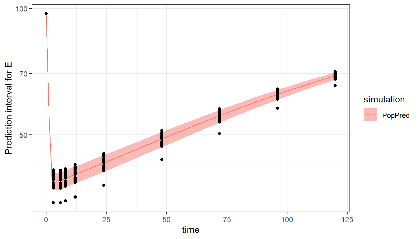
When using the plot_prediction() function, the output to display can be chosen with the output argument. In addition, a log-scale on the y-axis can be set with ylog=T. In this example, the simulation using the typical population parameters is shown as a prediction interval because of the different covariate value for each individual.
plot_prediction(saved_project = "ex4b_saved_project.mlxtran",
                output = "E",
                ylog   = T)
Using regressors
In this example, we consider a sequential PD model with fixed individual PK parameters given as regressors. The individual PK parameters are considered as known and part of the model information. They can be given in the regressor argument, which is a data frame with columns “id”, “time” and one column per parameter (i.e regressor). Note that even if the PK parameters are constant over time, a time column is necessary. If the names of the regressor columns in the dataset differ from the names in the model file (here Tlag_mode in the dataset and Tlag in the model), the names in the regressor argument must correspond to the names in the dataset. Make sure to use the same order in the input line of the model and in the data frame given as regressor argument in mlxDesignEval.
The structural model of this example is the following:
"[LONGITUDINAL]
input =  {IC50, Rin, kout, Tlag, ka, V, Cl}
Tlag = {use = regressor}
ka   = {use = regressor}
V    = {use = regressor}
Cl   = {use = regressor}

EQUATION:
Cc = pkmodel(Tlag,ka,V,Cl)
E_0 = Rin/kout
ddt_E= Rin*(1-Cc/(Cc+IC50)) - kout*E

OUTPUT:
output = E"
We define the regressor values in a data frame, by sampling values from lognormal distributions using the R function rlnorm:
proj5 <- system.file("extdata","warfarin_PKPDseq_project.mlxtran", package="mlxDesignEval")
nbIndiv <- 20
reg5 <- data.frame(id=1:nbIndiv,
                   time=0,
                   Tlag_mode=rlnorm(nbIndiv, meanlog = log(0.84), sdlog = 0.6),
                   ka_mode  =rlnorm(nbIndiv, meanlog = log(1.30), sdlog = 0.9),
                   V_mode   =rlnorm(nbIndiv, meanlog = log(7.85), sdlog = 0.2),
                   Cl_mode  =rlnorm(nbIndiv, meanlog = log(0.13), sdlog = 0.3))

res5a <- evaluate_design(project_file = proj5,
                        population_parameters = data.frame(IC50_pop=1.15,Rin_pop=5.2,kout_pop=0.05,omega_IC50=0.47,omega_Rin=0.013,omega_kout=0.016,a2=4),
                        output    = list(output="y2", data=data.frame(time=c(0, 6, 12, 24, 48, 72, 96, 120))),
                        treatment = list(data=data.frame(time=0, amount=5)),
                        regressor = reg5,
                        group     = list(size=nbIndiv))
print(res5a$RSE)
#>                   RSE
#> IC50_pop    11.661132
#> Rin_pop      6.131623
#> kout_pop     5.998700
#> omega_IC50  17.824290
#> omega_Rin  615.161979
#> omega_kout 387.536289
#> a2           6.373833
The regressors can also be defined in an external file, whose path is given as regressor argument:
write.csv(reg5, "reg_file.csv", row.names = F, quote = F)

res5b <- evaluate_design(project_file=proj5,
                        population_parameters = data.frame(IC50_pop=1.15,Rin_pop=5.2,kout_pop=0.05,omega_IC50=0.47,omega_Rin=0.013,omega_kout=0.016,a2=4),
                        output=list(output="y2", data=data.frame(time=c(0, 6, 12, 24, 48, 72, 96, 120))),
                        treatment=list(data=data.frame(time=0, amount=5)),
                        regressor = "reg_file.csv",
                        group=list(size=nbIndiv))
print(res5b$RSE)
#>                   RSE
#> IC50_pop    11.661132
#> Rin_pop      6.131623
#> kout_pop     5.998700
#> omega_IC50  17.824290
#> omega_Rin  615.161979
#> omega_kout 387.536289
#> a2           6.373833
If the regressor argument is not given, the regressor values from the Monolix project are used and a warning message is raised:
res5c <- evaluate_design(project_file=proj5,
                        population_parameters = data.frame(IC50_pop=1.15,Rin_pop=5.2,kout_pop=0.05,omega_IC50=0.47,omega_Rin=0.013,omega_kout=0.016,a2=4),
                        output=list(output="y2", data=data.frame(time=c(0, 6, 12, 24, 48, 72, 96, 120))),
                        treatment=list(data=data.frame(time=0, amount=5)),
                        group=list(size=nbIndiv))
#> [INFO] No regressor argument provided. The regressor information of the Monolix project's dataset will be used.
print(res5c$RSE)
#>                   RSE
#> IC50_pop    11.742700
#> Rin_pop      5.750078
#> kout_pop     5.648664
#> omega_IC50  17.984149
#> omega_Rin  572.327336
#> omega_kout 363.390609
#> a2           6.369380
Using multiple doses
Implementation of multiple doses is straightforward: instead of defining a data frame with a single dose line, we can define several dose lines. Note that both ODE-based models and macro-based models (e. with pkmodel()) are able to handle multiple doses.
trt6 <- list(data=data.frame(time=seq(0,144,by=24), amount=5))

res6 <- evaluate_design(project_file = system.file("extdata","theophylline_project.mlxtran", package="mlxDesignEval"),
                       population_parameters = data.frame(ka_pop=1.5,V_pop=0.45,Cl_pop=0.04, omega_ka=0.66, omega_V=0.12, omega_Cl=0.27, a=0.43, b=0.055),
                       output = list(output="CONC", data=data.frame(time=c(1,2,8,120,144))),
                       treatment = trt6,
                       group = list(size=20),
                       saved_project = "ex6_saved_project.mlxtran")
The multiple doses can be seen when plotting the model and design. To see well the profile of each dose, we increase the number of points to 500 for the time grid of the prediction.
plot_prediction(saved_project = "ex6_saved_project.mlxtran",
                plot = "PopPred",
                plot_grid = 500)
Using different types of administrations
Different types of administrations (e.g IV and oral) or different drugs can be distinguished by different administration identifiers, indicated with the adm keyword in administration macros of the model file (e.g iv(), oral() or depot()) and with the admID keyword in the design definition for mlxDesignEval.
We will use the following model. We decided to use adm=1 for IV doses which will be handled by the iv() macro and adm=2 for oral doses which will be handled by the oral() macro.
model <- inlineModel("
[INDIVIDUAL]
input = {F_pop, omega_F, ka_pop, omega_ka, V_pop, omega_V, k_pop, omega_k}

DEFINITION:
F = {distribution=logitNormal, typical=F_pop, sd=omega_F}
ka = {distribution=logNormal, typical=ka_pop, sd=omega_ka}
V = {distribution=logNormal, typical=V_pop, sd=omega_V}
k = {distribution=logNormal, typical=k_pop, sd=omega_k}

[LONGITUDINAL]
input = {F, ka, V, k, b}

PK:
compartment(cmt=1, amount=Ac)
iv(cmt=1, adm=1)
oral(cmt=1, adm=2, ka, p=F)
elimination(cmt=1, k)
Cc=Ac/V

OUTPUT:
output = Cc

DEFINITION:
Y = {distribution=normal, prediction=Cc, errorModel=proportional(b)}
")
We would like two use two arms (i.e groups):
-
arm 1: oral doses (PO) of 50mg every 24h
-
arm 2: one loading IV bolus dose of 75mg followed by 50 mg oral doses (PO) every 24h
Each treatment definition can contain only one admID value. For arm 2, we thus define two treatments (the loading IV dose and the oral maintenance doses) and combine them together within a list.
In addition, in order to be specific to each arm (i.e group), the treatments are given in the group argument, and not as direct input to the evaluate_design call.
trt_IV_arm2 <- list(data=data.frame(time=0, amount=75), admID=1)
trt_PO_arm2 <- list(data=data.frame(time=seq(from=24,to=120,by=24), amount=50), admID=2)
trt_arm1 <- list(data=data.frame(time=seq(from=0 ,to=120,by=24), amount=50), admID=2)
trt_arm2 <- list(trt_IV_arm2,trt_PO_arm2)
arm1 <- list(size=20, treatment=trt_arm1)
arm2 <- list(size=15, treatment=trt_arm2)

res7 <- evaluate_design(project_file = system.file("extdata","ivOral1_project.mlxtran", package="mlxDesignEval"),
                        population_parameters = data.frame(F_pop=0.68, ka_pop=1.03, V_pop=9.45, k_pop=0.028,
                   omega_F=0.45, omega_ka=0.32, omega_V=0.23, omega_k=0.2, b=0.15),
                        output = list(output="Y", data=data.frame(time=c(0.5,1,3,6,12,24,48,72,96,120,126,132,144,168))),
                        group = list(arm1,arm2))

print(res7$RSE)
#>                RSE
#> F_pop     4.812421
#> ka_pop    8.446183
#> V_pop     4.997499
#> k_pop     3.834462
#> omega_F  36.035168
#> omega_ka 21.720998
#> omega_V  16.243422
#> omega_k  14.397430
#> b         3.577206
Using occasions
Occasions denote different periods of time. They can be used to let covariates or individual parameters vary from occasion to occasion within a given individual. In order to use occasions, an occasion argument must be defined. Occasions can be the same for all individuals or the occasion structure can be different for each individual. In any case, the occasion information must be repeated in the definition of the treatment, output, covariate and regressors, and they must be the same for all elements.
Same occasions for all individuals
When the occasion structure is the same for all individuals, occasions are defined as a data frame with columns time (indicating the start time of the period) and occ (an integer changing for each new occasion). This occasion information is also repeated in the output, treatment and covariate elements.
In the example below we consider a (ka, V, Cl) model. Two different treatments are encoded via a covariate TREAT with can take values “A” or “B”, and there is an effect of the covariate TREAT on the volume V. The individuals receive first treatment A at time 0 and then treatment B 24h later. In order to let the covariate TREAT change over time, we will define occasions. The first occasion starts at time 0 and a second occasion starts at time 24.
The output spans from time 0 to 48h, with each time point having an occasion value consistent with the occasion definition. The occasion information is also repeated for the treatment and covariate definition. Note that if the occasions are defined as “common” (without “id” column), the covariates must also be the same for all individuals. If you want different covariates between individuals, use subject-specific occasions (see next section).
occ8 <- data.frame(time=c(0,24),occ=c(1,2))
out8 <- list(output="Y", data=data.frame(time=c(0.25, 0.5, 0.75, 1, 2, 3, 6, 8, 12, 23.9,
                                                24.25,24.5,24.75,25,26,27,30,32,36,48),
                                         occ=rep(c(1,2),each=10)))
trt8 <- list(data=data.frame(occ=c(1,2), time=c(0,24), amount=5))
cov8 <- data.frame(occ=c(1,2), TREAT=c("A","B"))

res8 <- evaluate_design(project_file=system.file("extdata","iov2_project.mlxtran", package="mlxDesignEval"),
                        population_parameters = data.frame(ka_pop=1.5,V_pop=0.45,Cl_pop=0.04, omega_ka=0.25, omega_V=0.09, gamma_V=0.20 , omega_Cl=0.20, beta_V_TREAT_B=-0.23, b=0.09, a=0.3),
                        output    = out8,
                        treatment = trt8,
                        covariate = cov8,
                        occasion  = occ8,
                        group = list(size=50),
                        saved_project = "ex8_saved_project.mlxtran")
print(res8$RSE)
#>                      RSE
#> ka_pop          4.002162
#> V_pop           3.279116
#> beta_V_TREAT_B 18.336283
#> Cl_pop          2.906709
#> omega_ka       12.595434
#> omega_V        48.599522
#> omega_Cl       10.561569
#> gamma_V        11.109939
#> a              12.863514
#> b               7.336758
The two occasions can be visualized:
plot_prediction(saved_project = "ex8_saved_project.mlxtran", plot = c("PopPred"))
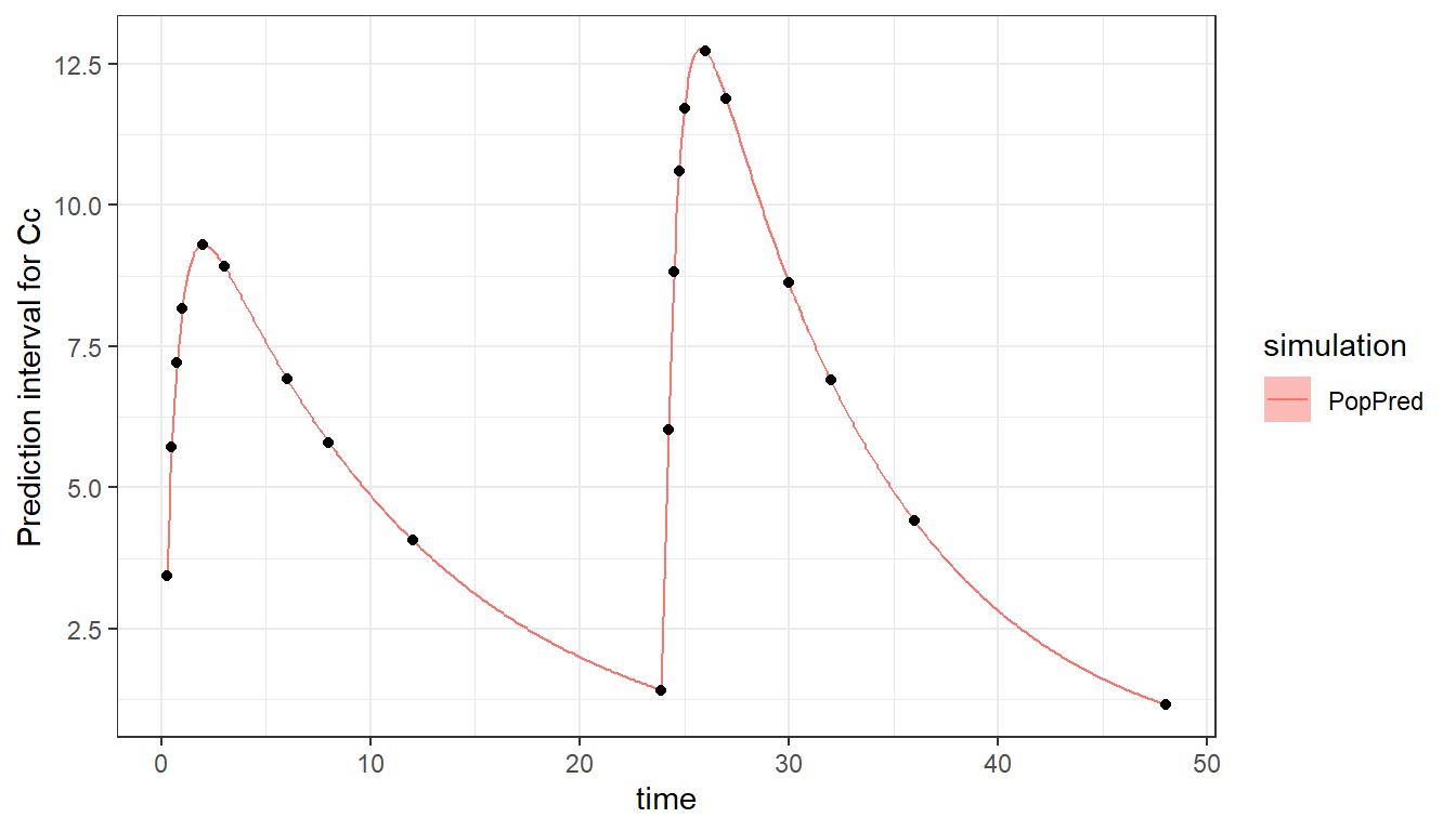
Note that if there is an overlap in the time of outputs or doses between occasion 1 and 2, a washout (reset) will be automatically applied between the two occasions. This is for instance the case if we list time 24 as being part of occasion 1 in the output definition. We then have an overlap between occasion 1 which goes up to time 24 because of the output, and occasion 2 which starts at time 24.
Different occasions for each individual
Several limitations of the “common” occasions shown in the previous sections can force us to use individual-specific occasions:
-
if we want to take into account covariates which vary from individual to individual: a common occasion element cannot be used because the occasions would also have to be common for the covariate element
-
if we want a different occasion structure for different arms: the occasion definition cannot be put within the group definition
In those two situations, using individual-specific occasions is a solution. This is done by adding an “id” column to the data frame defining the occasions to define the occasion structure of each individual. Note that the occasion structure for each individual can be the same if needed (as in the example below). As a consequence, we also need the same structure with “id” and “occ” columns in the definition of covariates, treatments, outputs and regressors.
Re-using the same example as above, we now would like to sample the treatments “A” and “B” randomly for each individual and each occasion.
nbIndiv <- 20
# covariates as data.frame with different covariate sequence for each id
cov9  <- data.frame(id  = rep(1:nbIndiv, each=2),
                    occ = rep(c(1,2), times=nbIndiv),
                    TREAT=sample(c("A","B"),nbIndiv*2, replace=T))
# occasion element must also be with column "id"
occ9  <- data.frame(id = rep(1:nbIndiv, each=2),
                    occ= rep(c(1,2),  times=nbIndiv),
                    time=rep(c(0,24), times=nbIndiv))
# output times must also be with a column "id"
out9  <- data.frame(id  =rep(1:nbIndiv, each=2*20),
                    occ =rep(rep(c(1,2),each=10), times=nbIndiv),
                    time=rep(c(0.25, 0.5, 0.75, 1, 2, 3, 6, 8, 12, 23.9, 24.25,24.5,24.75,25,26,27,30,32,36,48),times=nbIndiv))
# treatment  must also be with a column "id"
trt9  <- data.frame(id = rep(1:nbIndiv, each=2),
                    occ= rep(c(1,2), times=nbIndiv),
                    time=rep(c(0,24),times=nbIndiv),
                    amount=5)

res9  <- evaluate_design(project_file=system.file("extdata","iov2_project.mlxtran", package="mlxDesignEval"),
                         population_parameters = data.frame(ka_pop=1.5,V_pop=0.45,Cl_pop=0.04, omega_ka=0.25, omega_V=0.09, gamma_V=0.20 , omega_Cl=0.20, beta_V_TREAT_B=-0.23, b=0.09, a=0.3),
                         output    = list(output="Y", data=out9),
                         treatment = list(data=trt9),
                         covariate = cov9,
                         occasion  = occ9,
                         group     = list(size=nbIndiv))
print(res9$RSE)
#>                      RSE
#> ka_pop          6.319335
#> V_pop           5.375602
#> beta_V_TREAT_B 31.898350
#> Cl_pop          4.612375
#> omega_ka       19.855558
#> omega_V        76.877086
#> omega_Cl       16.819780
#> gamma_V        17.538315
#> a              20.553075
#> b              11.855196
Reusing a prior FIM
The FIM of a design with study 1 and study 2 is equal to the sum of the FIM of study 1 and the FIM of study 2. This property can be used to calculate the FIM of a first design with study 1, save it, and then calculate the FIM of a design with study 2 assuming that we already have the knowledge of study 1. This is done by calculating the FIM of study 2 and adding on top the previous FIM coming from the study 1. This way we take into account the prior knowledge coming from the first study.
We illustrate this by calculating first the FIM and RSEs for a design with 20 adults and dense sampling. The population parameters can be well estimated as shown by the low RSEs.
res10adult <- evaluate_design(project_file = system.file("extdata","theophylline_project.mlxtran", package="mlxDesignEval"),
                         population_parameters = data.frame(ka_pop=1.5,V_pop=0.45,Cl_pop=0.04, omega_ka=0.66, omega_V=0.12, omega_Cl=0.27, a=0.43, b=0.055),
                         output = list(output="CONC", data=data.frame(time=c(0.25, 0.5, 0.75, 2, 3, 6, 8, 12, 24))),
                         treatment = list(data=data.frame(time=0, amount=5)),
                         group = list(size=20))
print(res10adult)
#> $RSE
#>                RSE
#> ka_pop   15.300131
#> V_pop     3.309864
#> Cl_pop    6.431617
#> omega_ka 16.761370
#> omega_V  23.818950
#> omega_Cl 17.876194
#> a        27.118313
#> b        37.745735
#>
#> $OFV
#> [1] 54.78381
#>
#> $FIM
#>             ka_pop      V_pop     Cl_pop    omega_ka     omega_V     omega_Cl
#> ka_pop    19.25418  -34.13614     32.958  0.00000000    0.000000   0.00000000
#> V_pop    -34.13614 4594.41131   1936.741  0.00000000    0.000000   0.00000000
#> Cl_pop    32.95800 1936.74074 152025.769  0.00000000    0.000000   0.00000000
#> omega_ka   0.00000    0.00000      0.000 81.75341427    4.204951   0.06968215
#> omega_V    0.00000    0.00000      0.000  4.20495136 1246.432253   3.93752504
#> omega_Cl   0.00000    0.00000      0.000  0.06968215    3.937525 431.32246923
#> a          0.00000    0.00000      0.000  3.75718850   89.394608  23.60749579
#> b          0.00000    0.00000      0.000 19.79880253  571.579477  76.78708142
#>                    a           b
#> ka_pop      0.000000     0.00000
#> V_pop       0.000000     0.00000
#> Cl_pop      0.000000     0.00000
#> omega_ka    3.757188    19.79880
#> omega_V    89.394608   571.57948
#> omega_Cl   23.607496    76.78708
#> a         468.758612  2419.36853
#> b        2419.368533 14821.76261
If instead we consider a sparse sampling with 6 children (which have a lower clearance), the parameters are not well identifiable.
res10children <- evaluate_design(project_file = system.file("extdata","theophylline_project.mlxtran", package="mlxDesignEval"),
                          population_parameters = data.frame(ka_pop=1.5,V_pop=0.45,Cl_pop=0.02, omega_ka=0.66, omega_V=0.12, omega_Cl=0.27, a=0.43, b=0.055),
                          output = list(output="CONC", data=data.frame(time=c(2, 6, 24))),
                          treatment = list(data=data.frame(time=0, amount=5)),
                          group = list(size=6))
print(res10children$RSE)
#>                 RSE
#> ka_pop    47.579407
#> V_pop      6.996521
#> Cl_pop    12.916617
#> omega_ka 117.338776
#> omega_V   54.552409
#> omega_Cl  61.285609
#> a        474.833380
#> b        489.763647
Next we can add the prior information from the adult study and evaluate the pediatric design. This is the same as pooling the adult and pediatric data together. Note that the two studies must have the same parameters, such that the FIMs have the same dimensions and can be summed. As expected, the RSEs are now much better.
res10both <- evaluate_design(project_file = system.file("extdata","theophylline_project.mlxtran", package="mlxDesignEval"),
                             population_parameters = data.frame(ka_pop=1.5,V_pop=0.45,Cl_pop=0.02, omega_ka=0.66, omega_V=0.12, omega_Cl=0.27, a=0.43, b=0.055),
                             output = list(output="CONC", data=data.frame(time=c(2, 6, 24))),
                             treatment = list(data=data.frame(time=0, amount=5)),
                             prior_FIM = res10adult$FIM,
                             group = list(size=6))
print(res10both$RSE)
#>                RSE
#> ka_pop   14.525765
#> V_pop     2.958634
#> Cl_pop    9.060054
#> omega_ka 16.364011
#> omega_V  21.464511
#> omega_Cl 16.227422
#> a        26.823433
#> b        36.972761
Taking into account the uncertainty
When performing a design evaluation, the input population parameters might not be well known and we may want to take this uncertainty into account. To do so, we can either provide several sets of population parameters (e.g coming from a bootstrap run) or sample sets of population parameters from their uncertainty distribution.
With several sets of pop param
Instead of giving a single set of population parameters, it is possible to provide to the population_parameters argument a data frame where each row corresponds to a different set of population parameters. The RSEs will be calculated for each set and returned in a data frame.
pop11 <- data.frame(ka_pop=c(1.5,1.4, 1.37),V_pop=c(0.45,0.47, 0.47),Cl_pop=c(0.04,0.04,0.05),
                    omega_ka=c(0.66,0.70,0.57), omega_V=c(0.12,0.10,0.15), omega_Cl=c(0.27,0.53, 0.34),
                    a=c(0.43,0.46,0.32), b=c(0.055,0.06,0.052))

res11 <- evaluate_design(project_file = system.file("extdata","theophylline_project.mlxtran", package="mlxDesignEval"),
                         population_parameters = pop11,
                         output = list(output="CONC", data=data.frame(time=c(0.25, 0.5, 0.75, 2, 3, 6, 8, 12, 24))),
                         treatment = list(data=data.frame(time=0, amount=5)),
                         group = list(size=20))
print(res11$RSE)
#>               pop1      pop2      pop3
#> ka_pop   15.300131 16.274213 13.236389
#> V_pop     3.309864  3.107158  3.819804
#> Cl_pop    6.431617 12.112638  7.806978
#> omega_ka 16.761370 16.742406 16.880393
#> omega_V  23.818950 30.340353 20.354568
#> omega_Cl 17.876194 16.467213 16.653449
#> a        27.118313 27.488097 24.405370
#> b        37.745735 38.837875 31.494928
Sampling from the uncertainty distribution
To sample sets of population parameters, it is necessary to use a Monolix project with calculated standard errors. The RSEs and covariance matrix of the population parameters will be used to generate sets of population parameters. To use this option, set population_parameters as either "mlx_PopUncertainLin" (if the standard errors were calculated via linearization) or "mlx_PopUncertainSA" (if the standard errors were calculated via stochastic approximation). These keywords correspond to the names of the elements created when exporting a Monolix project to Simulx. In addition, we need to specify how many samples we want to use. This is done with the npop argument.
res12 <- evaluate_design(project_file = system.file("extdata","theophylline_project.mlxtran", package="mlxDesignEval"),
                         population_parameters = "mlx_PopUncertainLin",
                         output = list(output="CONC", data=data.frame(time=c(0.25, 0.5, 0.75, 2, 3, 6, 8, 12, 24))),
                         treatment = list(data=data.frame(time=0, amount=5)),
                         group = list(size=20),
                         npop = 10)
print(res12$RSE)
#>               pop1      pop2      pop3      pop4      pop5      pop6      pop7
#> ka_pop   15.253557 18.077113 13.696496 16.188484 12.001083 18.061451 15.596121
#> V_pop     3.799803  3.424792  1.852817  3.269098  3.786568  3.352879  2.931426
#> Cl_pop    6.592951  7.057110  6.754465  8.087088  6.272503  6.296316  6.274958
#> omega_ka 16.505588 16.498922 16.484062 16.456605 17.991996 16.534556 16.756398
#> omega_V  18.797524 21.470683 46.235009 19.723296 24.312975 24.381832 28.271826
#> omega_Cl 17.082230 17.661834 17.151021 16.668008 17.931779 18.569342 18.450811
#> a        38.983016 19.282775 21.320505 35.198841 31.512146 20.977024 19.261109
#> b        35.261217 81.057676 58.102260 37.954573 23.017494 64.444799 65.777754
#>               pop8      pop9     pop10
#> ka_pop   16.839982  9.574090 14.544449
#> V_pop     3.701175  4.171283  3.592729
#> Cl_pop    5.587853  6.042243  5.834398
#> omega_ka 16.840053 20.822772 16.823170
#> omega_V  21.772902 22.486645 19.803493
#> omega_Cl 18.866436 20.101201 17.432226
#> a        28.188069 28.358864 32.524233
#> b        30.256103 35.909578 26.384175
Parameter identifiability
mlxDesignEval can also be used to assess the identifiability of the population parameters, given a model and dataset, before launching a Monolix run. In this case, instead of considering a possible future trial design, we want to evaluate the identifiability of the population parameters with the design present in the dataset at hand. The procedure is the same as before, except that the design information is read directly from the Monolix dataset, and not given as separate arguments to the evaluate_design function. As the calculations are very fast, it allows to rapidly assess if the parameters are likely to be estimated with good confidence, before doing a full Monolix run which can take much longer depending on the dataset and model.
Identifiable model
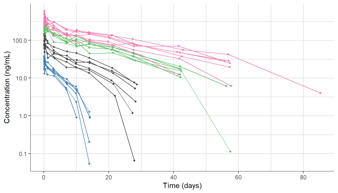
To illustrate this feature, we will use the dataset of a monoclonal antibody, which was administered by IV injection to healthy volunteers. The study comprises 4 single dose groups with 6 individuals each.
The plotted data displays the typical pattern of target-mediated drug disposition (TMDD) with a downward curvature at the end of the profiles.
To model this data, we first consider the simplest TMDD model, called Michaelis-Menten (MM) approximation, which contains a linear clearance term Cl and a non-linear clearance term with parameters Vm and Km. This model is available in the TMDD library.
We would like to assess if the parameters of the model will be identifiable given the design of our dataset. For this, we create a Monolix project with the dataset and the model. The initial parameter values must reasonably capture our data:
-
The fixed effects are set using the autoinit feature of Monolix
-
The standard deviation of the random effects “omegas” are set to 0.3 (i.e 30% IIV) which is a typical value for PK parameters
-
The proportional error term “b” is set to 0.15 (i.e 15%) which is also typical for PK data
These initial values are saved in the Monolix project.
To know if the population parameters will be identifiable, we run the evaluate_design function giving as only input the Monolix project. The design (treatment and output in this example) will be read from the Monolix dataset, and the population parameter values from the initial values of the Monolix project. Note that each individual can have a different design, as in any Monolix dataset.
res13a <- evaluate_design(project_file = system.file("extdata","TMDD_MM.mlxtran", package="mlxDesignEval"))
#> [INFO] No population_parameters argument provided and no valid Monolix results. The initial values of the monolix project will be used.
#> [INFO] No output argument provided. The observation times of the Monolix project's dataset will be used.
#> [INFO] No treatment argument provided. The treatment information of the Monolix project's dataset will be used.
#> [INFO] No group size argument provided. The number of individuals of the Monolix project will be used.
The predicted RSEs indicate that we expect all parameters to be identifiable, except maybe the omega_Km.
print(res13a$RSE)
#>                 RSE
#> V_pop      6.156582
#> Vm_pop    11.309332
#> Km_pop    30.070351
#> Cl_pop    12.600238
#> Q_pop     11.299469
#> V2_pop    10.657861
#> omega_V   14.772046
#> omega_Vm  23.201676
#> omega_Km 121.372247
#> omega_Cl  26.632895
#> omega_Q   47.496784
#> omega_V2  28.940379
#> b          4.806126
Non-identifiable model
Next we consider a more complex TMDD model, the quasi-equilibrium (QE) approximation, which contains 2 additional parameters. Again, the fixed effects are set using the autoinit option, all omegas are set to 0.3 and b=0.15.
res13b <- evaluate_design(project_file = system.file("extdata","TMDD_QE.mlxtran", package="mlxDesignEval"))
#> [INFO] No population_parameters argument provided and no valid Monolix results. The initial values of the monolix project will be used.
#> [INFO] No output argument provided. The observation times of the Monolix project's dataset will be used.
#> [INFO] No treatment argument provided. The treatment information of the Monolix project's dataset will be used.
#> [INFO] No group size argument provided. The number of individuals of the Monolix project will be used.
This time we see that several parameters have very high RSEs, indicating their unidentifiability. It is the case for KD (binding constant) and kint (internalization rate). This is consistent with the fact that these parameters impact the model prediction in a section of the concentration-time profile in which no measurements have been done, see the scheme in “Overview of the model hierarchy” of our TMDD library.
print(res13b$RSE)
#>                     RSE
#> V_pop          7.517692
#> kint_pop    4164.276648
#> KD_pop      4222.913686
#> ksyn_pop      13.287400
#> R0_pop       219.895430
#> Cl_pop        12.131983
#> Q_pop         13.758743
#> V2_pop        11.176583
#> omega_V       14.791965
#> omega_kint 17414.649006
#> omega_KD   17791.352456
#> omega_ksyn    25.815478
#> omega_R0     970.494719
#> omega_Cl      24.830872
#> omega_Q       53.500467
#> omega_V2      29.089632
#> b              4.820968
Sensitivity to initial values
The evaluate_design procedure is quite sensitive to the initial values set in the Monolix project, in particular the fixed effects.
Let’s set the initial value of Vm_pop to 0.1 (instead of 1.6 in the first example). With this Vm_pop value, the downward curvature is not visible anymore in the model prediction:
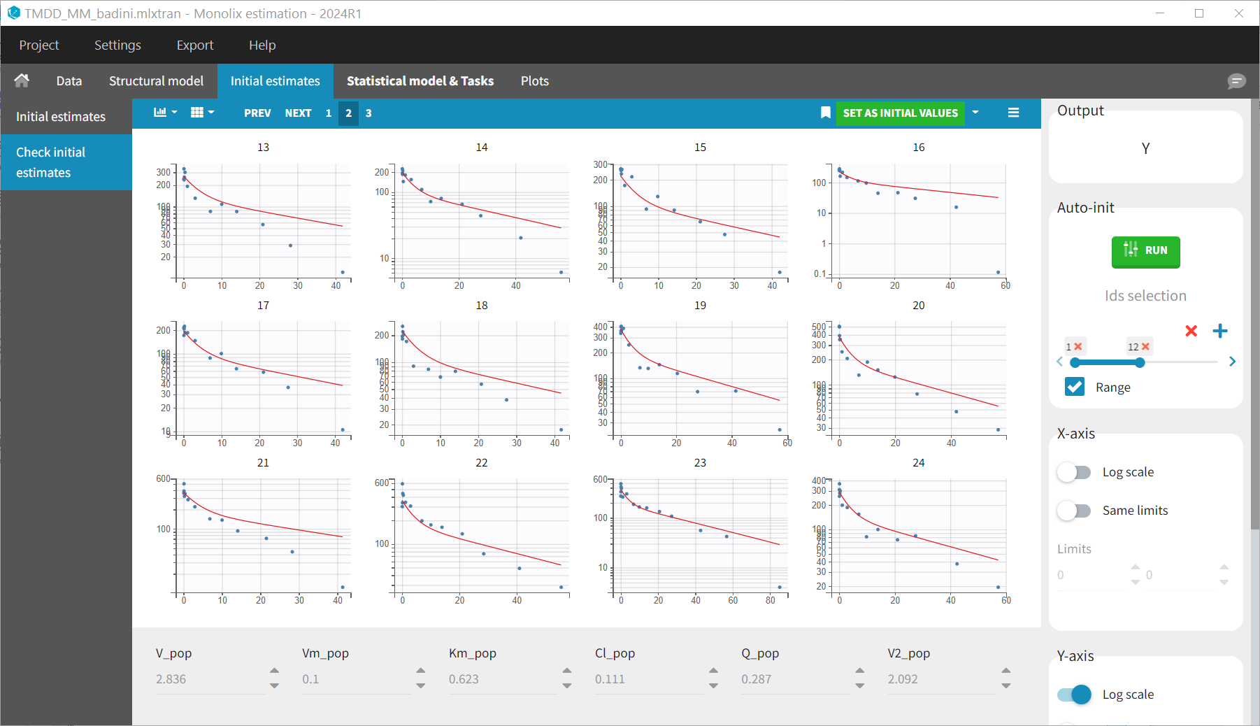
As a consequence Km and Vm appear as unidentifiable while it is actually not the case.
res13c <- evaluate_design(project_file = system.file("extdata","TMDD_MM_badini.mlxtran", package="mlxDesignEval"))
#> [INFO] No population_parameters argument provided and no valid Monolix results. The initial values of the monolix project will be used.
#> [INFO] No output argument provided. The observation times of the Monolix project's dataset will be used.
#> [INFO] No treatment argument provided. The treatment information of the Monolix project's dataset will be used.
#> [INFO] No group size argument provided. The number of individuals of the Monolix project will be used.
print(res13c$RSE)
#>                     RSE
#> V_pop          6.163286
#> Vm_pop       473.257858
#> Km_pop      9691.145443
#> Cl_pop        17.702429
#> Q_pop         12.792693
#> V2_pop        11.851793
#> omega_V       14.778137
#> omega_Vm    6556.015050
#> omega_Km 2787984.138326
#> omega_Cl      23.676266
#> omega_Q       62.737726
#> omega_V2      36.568353
#> b              4.732498
Conclusion
When using mlxDesignEval for parameter identifiability assessment, high RSEs can indicate unidentifiable parameters or bad initial values. Always make sure that the initial value is such that the impact of the parameter on the model prediction is visible if the parameter value is slightly changed.

